Merge pull request #107 from jlizier/course

Merging course branch into master

README.md

@@ -1,6 +1,6 @@
 # Java Information Dynamics Toolkit (JIDT)
 
-Copyright (C) 2012-2014 [Joseph T. Lizier](http://lizier.me/joseph/); 2014-2016 [Joseph T. Lizier](http://lizier.me/joseph/) and Ipek Özdemir; 2017- [Joseph T. Lizier](http://lizier.me/joseph/), Ipek Özdemir and [Pedro Mediano](https://www.doc.ic.ac.uk/~pam213/)
+Copyright (C) 2012- [Joseph T. Lizier](http://lizier.me/joseph/); 2014- Ipek Özdemir; 2017- [Pedro Mediano](https://www.doc.ic.ac.uk/~pam213/); 2019- Emanuele Crosato, Sooraj Sekhar, Oscar Huaigu Xu; 2020- [Julio Correa Rios](http://linkedin.com/in/juliocorrearios); 2021- [Isabelle De Backer](https://www.linkedin.com/in/isabelledebacker/); 2022- [David Shorten](https://scholar.google.com/citations?user=ggF3Lt4AAAAJ&hl=en)
 
 *JIDT* provides a stand-alone, open-source code Java implementation (also usable in [Matlab, Octave](../../wiki/UseInOctaveMatlab), [Python](../../wiki/UseInPython), [R](../../wiki/UseInR), [Julia](../../wiki/UseInJulia) and [Clojure](../../wiki/UseInClojure)) of information-theoretic measures of distributed computation in complex systems: i.e. information storage, transfer and modification.
 
@@ -8,19 +8,25 @@ JIDT includes implementations:
  * principally for the measures **transfer entropy**, **mutual information**, and their conditional variants, as well as **active information storage**, entropy, etc;
  * for both _discrete_ and _continuous_-valued data;
  * using various types of estimators (e.g. _Kraskov-Stögbauer-Grassberger estimators_, _box-kernel estimation_, _linear-Gaussian_),
-as described in full at ImplementedMeasures.
+as described in full at [ImplementedMeasures](../../wiki/ImplementedMeasures).
+
+JIDT is easy to use:
+ * It ships with a **GUI application** -- the [AutoAnalyser](../../wiki/AutoAnalyser), see picture below -- to facilitate point-and-click analysis, as well as code template generation for more complex analysis.
+ * We provide **short video lectures** and corresponding slides in a (beta) [Course](../../wiki/Course) on how to understand using information-theoretic tools to analyse complex systems, and to implement such analysis with JIDT.
 
 JIDT is distributed under the [GNU GPL v3 license](http://www.gnu.org/licenses/gpl.html) (or later).
 
 # Getting started
 
- 1. [Download](../../wiki/Downloads) and [Installation](../../wiki/Installation) is very easy!
-   1. _Quick start_: download the latest [v1.4 full distribution](http://lizier.me/joseph/software/jidt/download.php?file=infodynamics-dist-1.4.zip) (suitable for all platforms) and see the readme.txt file therein.
- 1. [Documentation](../../wiki/Documentation) including: the paper describing JIDT at [arXiv:1408.3270](http://arxiv.org/abs/1408.3270) (distributed with the toolkit), a [Tutorial](../../wiki/Tutorial), and [Javadocs (v1.4 here)](http://lizier.me/joseph/software/jidt/javadocs/v1.4/);
- 1. [Demos](../../wiki/Demos) are included with the full distribution, including a [GUI app](../../wiki/AutoAnalyser) for automatic analysis and code generation (see picture below), [simple java demos](../../wiki/SimpleJavaExamples) and [cellular automata (CA) demos](../../wiki/CellularAutomataDemos).
-  1. These Java tools can easily be used in [Matlab/Octave](../../wiki/OctaveMatlabExamples), [Python](../../wiki/PythonExamples), [R](../../wiki/R_Examples), [Julia](../../wiki/JuliaExamples) and [Clojure](../../wiki/Clojure_Examples)! (click on each language here for examples)
+1. [Download](../../wiki/Downloads) and [Installation](../../wiki/Installation) is very easy!
+    1. _Quick start_: take a `git clone` (then build via [AntScripts](../../wiki/AntScripts)) OR download the latest [v1.6.1 full distribution](https://lizier.me/joseph/software/jidt/download.php?file=infodynamics-dist-1.6.1.zip) (suitable for all platforms) and see the readme.txt file therein.
+1. [Documentation](../../wiki/Documentation) including: the paper describing JIDT at [arXiv:1408.3270](http://arxiv.org/abs/1408.3270) (distributed with the toolkit), a (beta) [Course](../../wiki/Course) including short video lectures and a shorter [Tutorial](../../wiki/Tutorial), and [Javadocs (v1.6.1 here)](https://lizier.me/joseph/software/jidt/javadocs/v1.6.1/);
+1. [Demos](../../wiki/Demos) are included with the full distribution, including a [GUI app](../../wiki/AutoAnalyser) for automatic analysis and code generation (see picture below), [simple java demos](../../wiki/SimpleJavaExamples) and [cellular automata (CA) demos](../../wiki/CellularAutomataDemos).
+    1. These Java tools can easily be used in [Matlab/Octave](../../wiki/OctaveMatlabExamples), [Python](../../wiki/PythonExamples), [R](../../wiki/R_Examples), [Julia](../../wiki/JuliaExamples) and [Clojure](../../wiki/Clojure_Examples)! (click on each language here for examples)
 
-![Computing in the GUI app image](https://raw.githubusercontent.com/jlizier/jidt/master/web/AutoAnalyserGUI-2-Compute.png)
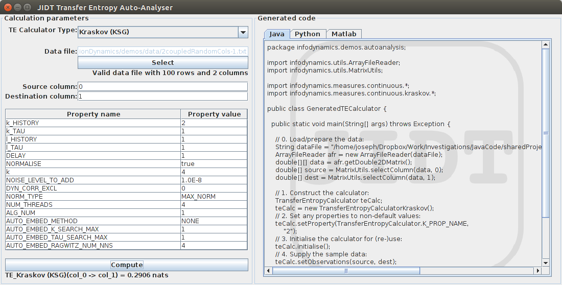
+[![Computing in the GUI app image](https://raw.githubusercontent.com/jlizier/jidt/master/web/AutoAnalyserGUI-2-Compute.png)](../../wiki/AutoAnalyser)
+
+[![Course and video lectures](https://raw.githubusercontent.com/jlizier/jidt/master/web/YouTubePlaylist.png)](../../wiki/Course)
 
 For further information or announcements:
  * Join our discussion group: http://groups.google.com/d/forum/jidt-discuss
@@ -39,6 +45,28 @@ See other [PublicationsUsingThisToolkit](../../wiki/PublicationsUsingThisToolkit
 
 # News
 
+_22/08/2023_ - New full distribution files available for **release v1.6.1**; Changes for v1.6.1 include:
+Minor updates to supporting use in Python, including virtual environments;
+Minor tweaks to fish schooling examples (mostly comments).
+
+_5/09/2022_ - New full distribution files available for **release v1.6**; Changes for v1.6 include:
+Adding Flocking/Schooling/Swarming demo;
+Included Pedro's code on IIT and O-/S-Information measures;
+Spiking TE estimator added from David;
+Fixed up AutoAnalyser to work well for Python3 and numpy;
+Links to lecture videos included in the beta wiki for the course;
+Added rudimentary effective network inference (simplified version of the IDTxl full algorithm) in demos/octave/EffectiveNetworkInference;
+
+_26/11/2018_ - New jar and full distribution files available for **release v1.5**; Changes for v1.5 include:
+Added GPU (cuda) capability for KSG Conditional Mutual Information calculator (proper documentation to come), brief [wiki page](../../wiki/GPU) and unit tests included;
+Added auto-embedding for TE/AIS with multivariate KSG, and univariate and multivariate Gaussian estimator (plus unit tests), for Ragwitz criteria and Maximum bias-corrected AIS, and also added Maximum bias corrected AIS and TE to handle source embedding as well;
+Kozachenko entropy estimator adds noise to data by default;
+Added bias-correction property to Gaussian and Kernel estimators for MI and conditional MI, including with surrogates (only option for kernel);
+Enabled use of different bases for different variables in MI discrete estimator;
+All new above features enabled in AutoAnalyser;
+Added drop-down menus for parameters in AutoAnalyser;
+Included long-form lecture slides in course folder;
+
 _26/11/2017_ - New jar and full distribution files available for **release v1.4**; Changes for v1.4 include:
 Major expansion of functionality for AutoAnalysers: adding Launcher applet and capability to double click jar to launch, added Entropy, CMI, CTE and AIS AutoAnalysers, also added binned estimator type, added all variables/pairs analysis, added statistical significance analysis, and ensured functionality of generated Python code with Python3;
 Added GPU (cuda) capability for KSG Mutual Information calculator (proper documentation and wiki page to come), including unit tests;
@@ -122,3 +150,11 @@ _19/11/2012_ - New jar and full distribution files available for v0.1.2, includi
 _31/10/2012_ - Jar and full distribution files available for v0.1.1 (first distribution)
 
 _7/5/2012_ - JIDT project created and code uploaded
+
+# Acknowledgements
+
+This project has been supported by funding through:
+* Australian Research Council Discovery Early Career Researcher Award (DECRA) "Relating function of complex networks to structure using information theory", J.T. Lizier, 2016-19 DE160100630
+* Universities Australia - Deutscher Akademischer Austauschdienst (German Academic Exchange Service) UA-DAAD Australia-Germany Joint Research Co-operation grant "Measuring neural information synthesis and its impairment", Wibral, Lizier, Priesemann, Wollstadt, Finn, 2016-17
+* University of Sydney Research Accelerator (SOAR) Fellowship 2019 Scheme, J.T. Lizier (CI), 2019-2020
+* Australian Research Council Discovery Project "Large-scale computational modelling of epidemics in Australia: analysis, prediction and mitigation", M. Prokopenko, P. Pattison, M. Gambhir, J.T. Lizier, M. Piraveenan, 2016-19 DP160102742

build.xml

@@ -5,12 +5,13 @@
 	</description>
 	
 	<!-- set global properties for this build -->
-	<property name="version" value="1.4"/>
+	<property name="version" value="1.6.1"/>
 	<property name="mainfilename" value="infodynamics"/>
 	<property name="jarplainname" value="${mainfilename}.jar" />
 	<property name="jarversiondistnamezip" value="${mainfilename}-jar-${version}.zip" />
 	<property name="distname" value="${mainfilename}-dist-${version}" />
 	<property name="distnamezip" value="${distname}.zip" />
+	<property name="distnametargz" value="${distname}.tar.gz" />
 	<property name="src" location="java/source"/>
 	<property name="cudasrc" location="cuda"/>
 	<property name="bin" location="bin"/>
@@ -42,17 +43,17 @@
 
 	<!-- Compile the java toolkit -->
 	<target name="compile" depends="init" description="compile the source">
-		<!-- Compile to Java 6 to provide compatibility for users with older JREs.
+		<!-- Compile to Java 8 to provide compatibility for users with older JREs.
 		     Caveat: The flags here only check the language compatibility, but
-		     may still use newer libraries which may cause issues for users with JDK 6.
-		     Indeed, one gets the warning: "bootstrap class path not set in conjunction with -source 1.6"
+		     may still use newer libraries which may cause issues for users with JDK 8.
+		     Indeed, one gets the warning: "bootstrap class path not set in conjunction with -source 1.8"
 		     To fix this, one would use the bootstrap classpath to point our JDK to an rt.jar
-		     for Java 6. 
-		     At this stage, I'm sure I'm not using new library calls from Java 7/8, so we can
-		     ignore the warning, and I don't want to bother installing Java 7 just to compile
-		     like this. I'll endeavour not to use JDK 8 libraries so as not to cause
+		     for Java 8. 
+		     At this stage, I'm sure I'm not using new library calls from Java 9+, so we can
+		     ignore the warning, and I don't want to bother installing newer Java just to compile
+		     like this. I'll endeavour not to use JDK 9+ libraries so as not to cause
 		     any issues here ... -->
-		<javac srcdir="${src}" destdir="${bin}" includeAntRuntime="false" target="1.6" source="1.6">
+		<javac srcdir="${src}" destdir="${bin}" includeAntRuntime="false" target="1.8" source="1.8" encoding="UTF8">
 			<classpath refid="apache-classpath"/>
 		</javac>
 
@@ -115,12 +116,12 @@
 	<target name="javadocs" depends="compile" description="Make the javadocs for the toolkit">
 		<delete dir="${javadocsdir}"/>
 		<javadoc destdir="${javadocsdir}">
-			<fileset dir="${src}">
-				<include name="**/*.java"/>
-				<exclude name="infodynamics/demos/**/*.java"/>
-				<exclude name="**/commonsmath3/*.java"/>
-				<exclude name="**/commonsmath3/**/*.java"/>
-			</fileset>
+			<packageset dir="${src}">
+				<include name="**"/>
+				<exclude name="infodynamics/demos/**"/>
+				<exclude name="**/commonsmath3/*"/>
+				<exclude name="**/commonsmath3/**"/>
+			</packageset>
 		</javadoc>
 		<!-- Change some of the style in the javadocs css for our lists: -->
 		<concat destfile="${javadocsdir}/stylesheet.css" append="true">
@@ -148,6 +149,7 @@
 		<delete file="demos/clojure/project.clj"/>
 		<delete file="${jarversiondistnamezip}"/>
 		<delete file="${distnamezip}"/>
+		<delete file="${distnametargz}"/>
 		<delete file="${jarplainname}"/>
 		<delete>
 			 <fileset dir="demos/AutoAnalyser" includes="GeneratedCalculator.*"/>
@@ -175,7 +177,7 @@
 	<!-- Compile and jar the toolkit with debug symbols -->
 	<target name="debug" depends="init" description="compile and jar with debug symbols">
 		<echo message="Compiling for debug"/>
-		<javac srcdir="${src}" destdir="${bin}" includeAntRuntime="false" target="1.6" source="1.6" debug="true">
+		<javac srcdir="${src}" destdir="${bin}" includeAntRuntime="false" target="1.7" source="1.7" debug="true">
 			<classpath refid="apache-classpath"/>
 		</javac>
 
@@ -293,23 +295,30 @@
 		</zip>
 	</target>
 	
-	<!-- Developer build - builds everything and makes the full distribution file -->
+	<!-- Developer build - builds everything and makes the full distribution file in zip and tar.gz -->
 	<target name="dist" depends="jar,junit,javadocs,readmefiles" description="developer: generate the full distribution">
 		<echo message="${ant.project.name}: ${ant.file}"/>
 		<zip destfile="${distnamezip}">
 			<fileset file="build.xml"/>
-			<fileset file="${jarplainname}"/>
+			<zipfileset file="${jarplainname}" filemode="755"/>
 			<fileset file="license-gplv3.txt"/>
 			<fileset file="readme.txt"/>
 			<fileset file="InfoDynamicsToolkit.pdf"/>
 			<fileset file="JIDT-logo.png" erroronmissingdir="false"/> <!-- This file is missing in full repository versions -->
 			<fileset file="${versionfile}"/>
 			<zipfileset dir="java" includes="**/*.java" prefix="java"/>
-			<zipfileset dir="demos" includes="**/*.*,**/*" excludes="clojure/deploy,clojure/deploy/*.*,python/*.pyc" prefix="demos"/>
+			<zipfileset dir="demos" includes="**/*.*,**/*" excludes="clojure/deploy,clojure/deploy/*.*,python/*.pyc,**/*.sh,**/*.bat" prefix="demos"/>
+			<zipfileset dir="demos" includes="**/*.sh,**/*.bat" prefix="demos" filemode="755"/> <!-- Do these separately to get executable permissions -->
 			<zipfileset dir="javadocs" includes="**/*.*,**/*" prefix="javadocs"/>
 			<zipfileset dir="notices" includes="**/*.*,**/*" prefix="notices"/>
-			<zipfileset dir="tutorial" prefix="tutorial"/>
+			<zipfileset dir="cuda" prefix="cuda" excludes="benchmark.sh"/>
+			<zipfileset dir="cuda" prefix="cuda" includes="benchmark.sh" filemode="755"/> <!-- Do this separately to get executable permissions -->
+			<zipfileset dir="course" prefix="course"/>
+			<zipfileset dir="tutorial" prefix="tutorial"/> <!-- Get rid of this when tutorial is subsumed in course... -->
 			<zipfileset dir="web" includes="JIDT-logo.png" prefix="" erroronmissingdir="false"/> <!-- This file is missing in zip dist versions -->
 		</zip>
+		<tar destfile="${distnametargz}" compression="gzip" longfile="posix"> <!-- for longfiles could also use "gnu" but apparently is slightly less widely supported -->
+			<zipfileset src="${distnamezip}"/>
+		</tar>
 	</target>
 </project>

course/Module01-Entropy/MatlabSimpleFunctions/completed/conditionalentropy.m

@@ -0,0 +1,43 @@
+% function conditionalentropy(p)
+%
+% Computes the conditional Shannon entropy over all outcomes x of a random
+%  variable X, given outcomes y of a random variable Y.
+%  Probability matrix p(x,y) is given for each candidate outcome
+%  (x,y).
+%
+% Inputs:
+% - p - 2D probability distribution function over all outcomes (x,y).
+%       p is a matrix over all combinations of x and y,
+%	where p(1,3) gives the probability of the first symbol of variable
+%	x co-occuring with the third symbol of variable y.
+%       E.g. p = [0.2, 0.3; 0.1, 0.4]. The sum over p must be 1.
+%
+% Outputs:
+% - result - conditional Shannon entropy of X given Y
+% 
+% Copyright (C) 2017, Joseph T. Lizier
+% Distributed under GNU General Public License v3
+%
+
+function result = conditionalentropy(p)
+
+	% Should we check any potential error conditions on the input?
+	% a. Should we check p is a matrix, not a vector?
+	% assert(~isvector(p));
+	% Actually we won't since a vector would be valid if one variable only ever took one value
+	% b. Check that the probabilities normalise to 1:
+	% assert(sum(p(:)) == 1);
+	assert(abs(sum(p(:)) - 1) < 0.0000001); % Will work for any dimensionality, and handles numerical rounding errors
+
+	% We need to compute H(X,Y) - H(Y):
+	% 1. joint entropy:
+	H_XY = jointentropy(p);
+	% 2. marginal entropy of Y:
+	%  But how to get p_y???
+	p_y = sum(p,1); % Since y changes along the columns, summing over the x's (dimension 1 argument in the sum) will just return p(y)
+	H_Y = entropy(p_y);
+	
+	result = H_XY - H_Y;
+	
+end
+

course/Module01-Entropy/MatlabSimpleFunctions/completed/conditionalentropyempirical.m

@@ -0,0 +1,49 @@
+% function conditionalentropyempirical(xn,yn)
+%
+% Computes the conditional Shannon entropy over all samples xn of a random
+%  variable X, given samples yn of a random variable Y.
+%
+% Inputs:
+% - xn - matrix of samples of outcomes x. May be a 1D vector of samples, or
+%        a 2D matrix, where each row is a vector sample for a multivariate X.
+% - yn - matrix of samples of outcomes x. May be a 1D vector of samples, or
+%        a 2D matrix, where each row is a vector sample for a multivariate Y.
+%        Must have the same number of rows as X.
+%
+% Outputs:
+% - result - conditional Shannon entropy of X given Y
+% 
+% Copyright (C) 2017, Joseph T. Lizier
+% Distributed under GNU General Public License v3
+%
+
+function result = conditionalentropyempirical(xn,yn)
+
+	% Should we check any potential error conditions on the input?
+	if (isvector(xn))
+		% Convert it to column vector if not already:
+		if (size(xn,1) == 1)
+			% xn has only one row:
+			xn = xn'; % Transpose it so it is only column
+		end
+	end
+	if (isvector(yn))
+		% Convert it to column vector if not already:
+		if (size(yn,1) == 1)
+			% yn has only one row:
+			yn = yn'; % Transpose it so it is only column
+		end
+	end
+	% Check that their number of rows are the same:
+	assert(size(xn,1) == size(yn,1));
+
+	% We need to compute H(X,Y) - H(X):
+	% 1. joint entropy:
+	H_XY = jointentropyempirical([xn, yn]);
+	% 2. marginal entropy of Y: (calling 'joint' in case yn is multivariate)
+	H_Y = jointentropyempirical(yn);
+	
+	result = H_XY - H_Y;
+	
+end
+

course/Module01-Entropy/MatlabSimpleFunctions/completed/conditionalmutualinformation.m

@@ -0,0 +1,63 @@
+% function conditionalmutualinformation(p)
+%
+% Computes the mutual information over all outcomes x of a random
+%  variable X with outcomes y of a random variable Y, conditioning on 
+%  outcomes z of a random variable Z.
+%  Probability matrix p(x,y,z) is given for each candidate outcome
+%  (x,y,z).
+%
+% Inputs:
+% - p - 3D probability distribution function over all outcomes (x,y,z).
+%       p is a matrix over all combinations of x and y and z,
+%	where p(1,3,2) gives the probability of the first symbol of variable
+%	x co-occuring with the third symbol of variable y and the second
+%	symbol of z.
+%       The sum over p must be 1.
+%       E.g.:
+%         p(:,:,1) = [0.114286, 0.171429; 0.057143, 0.228571];
+%         p(:,:,2) = [0.171429, 0.114286; 0.028571, 0.114286];
+%
+% Outputs:
+% - result - mutual information of X with Y given Z
+% 
+% Copyright (C) 2017, Joseph T. Lizier
+% Distributed under GNU General Public License v3
+%
+
+function result = conditionalmutualinformation(p)
+
+	% Should we check any potential error conditions on the input?
+	% a. Should we check p is a 3D matrix, not a vector or 2D matrix?
+	% assert(~isvector(p));
+	% Actually we won't since a vector/2D matrix would be valid if one/two variable only ever took one value
+	% b. Check that the probabilities normalise to 1:
+	% assert(sum(p(:)) == 1);
+	assert(abs(sum(p(:)) - 1) < 0.0000001); % Will work for any dimensionality, and handles numerical rounding errors
+
+	% We need to compute H(X|Z) + H(Y|Z) - H(X,Y|Z).
+	% But our conditional entropy calculator won't do H(X,Y|Z) since it doesn't accept a joint probability for X,Y.
+	% So, easier to rewrite as:
+	%  H(X,Z) - H(Z) + H(Y,Z) - H(Z) - H(X,Y,Z) + H(Z)
+	%  = H(X,Z) - H(Z) + H(Y,Z) - H(X,Y,Z)
+	% 1. joint entropy:
+	H_XYZ = jointentropy(p);
+	% 2. entropy of X,Z:
+	%  But how to get p_xz???
+	% Sum p over the y's (dimension 2 argument in the sum) will just return p(x,z) terms. Won't be a 2D array, but fine to compute entropy on
+	p_xz = sum(p,2);
+	H_XZ = jointentropy(p_xz);
+	% 3. entropy of Y,Z:
+	%  But how to get p_yz???
+	% Sum p over the x's (dimension 1 argument in the sum) will just return p(y,z) terms. Won't be a 2D array, but fine to compute entropy on
+	p_yz = sum(p,1);
+	H_YZ = jointentropy(p_yz);
+	% 4. marginal entropy of Z:
+	%  But how to get p_z???
+	% Sum p_xz over the x's (dimension 1 argument in the sum) will just return p(z) terms. Won't be a 1D array, but fine to compute entropy on
+	p_z = sum(p_xz,1); 
+	H_Z = jointentropy(p_z);
+	
+	result = H_XZ - H_Z + H_YZ - H_XYZ;
+	
+end
+

course/Module01-Entropy/MatlabSimpleFunctions/completed/conditionalmutualinformationempirical.m

@@ -0,0 +1,72 @@
+% function conditionalmutualinformationempirical(xn,yn,zn)
+%
+% Computes the mutual information over all samples xn of a random
+%  variable X with samples yn of a random variable Y, conditioning on 
+%  samples zn of a random variable Z.
+%
+% Inputs:
+% - xn - matrix of samples of outcomes x. May be a 1D vector of samples, or
+%        a 2D matrix, where each row is a vector sample for a multivariate X.
+% - yn - matrix of samples of outcomes y. May be a 1D vector of samples, or
+%        a 2D matrix, where each row is a vector sample for a multivariate Y.
+%        Must have the same number of rows as X.
+% - zn - matrix of samples of outcomes z. May be a 1D vector of samples, or
+%        a 2D matrix, where each row is a vector sample for a multivariate Z
+%        which will be conditioned on.
+%        Must have the same number of rows as X.
+%
+% Outputs:
+% - result - conditional mutual information of X with Y, given Z
+% 
+% Copyright (C) 2017, Joseph T. Lizier
+% Distributed under GNU General Public License v3
+%
+
+function result = conditionalmutualinformationempirical(xn,yn,zn)
+
+	% Should we check any potential error conditions on the input?
+	if (isvector(xn))
+		% Convert it to column vector if not already:
+		if (size(xn,1) == 1)
+			% xn has only one row:
+			xn = xn'; % Transpose it so it is only column
+		end
+	end
+	if (isvector(yn))
+		% Convert it to column vector if not already:
+		if (size(yn,1) == 1)
+			% yn has only one row:
+			yn = yn'; % Transpose it so it is only column
+		end
+	end
+	if (isvector(zn))
+		% Convert it to column vector if not already:
+		if (size(zn,1) == 1)
+			% zn has only one row:
+			zn = zn'; % Transpose it so it is only column
+		end
+	end
+	% Check that their number of rows are the same:
+	assert(size(xn,1) == size(yn,1));
+	assert(size(xn,1) == size(zn,1));
+
+	% We need to compute H(X|Z) + H(Y|Z) - H(X,Y|Z):
+	% 1. conditional joint entropy:
+	H_XY_given_Z = conditionalentropyempirical([xn, yn], zn);
+	% 2. conditional entropy of Y:
+	H_Y_given_Z = conditionalentropyempirical(yn, zn);
+	% 3. conditional entropy of X:
+	H_X_given_Z = conditionalentropyempirical(xn, zn);
+	
+	result = H_X_given_Z + H_Y_given_Z - H_XY_given_Z;
+
+	% Alternatively, note that we could compute I(X;Y,Z) - I(X;Z)
+	% 1. joint MI:
+	% I_X_YZ = mutualinformationempirical(xn, [yn, zn]);
+	% 2. MI just from Z:
+	% I_X_Z = mutualinformationempirical(xn, zn);
+	% Then:
+	% result = I_X_YZ - I_X_Z;
+
+end
+

course/Module01-Entropy/MatlabSimpleFunctions/completed/entropy.m

@@ -0,0 +1,43 @@
+% function entropy(p)
+%
+% Computes the Shannon entropy over all outcomes x of a random variable
+%  X with probability vector p(x) for each candidate outcome x.
+%
+% Inputs:
+% - p - probability distribution function over all outcomes x.
+%       p is a vector, e.g. p = [0.25, 0.75], the sum over which must be 1.
+%
+% Outputs:
+% - result - Shannon entropy of the probability distribution p
+% 
+% Copyright (C) 2017, Joseph T. Lizier
+% Distributed under GNU General Public License v3
+%
+
+function result = entropy(p)
+
+	% Should we check any potential error conditions on the input?
+	% assert(sum(p(:)) == 1);
+	assert(abs(sum(p(:)) - 1) < 0.0001); % Will work for any dimensionality, and handles numerical rounding errors
+	assert(~any(p(:) > 1));
+	assert(~any(p(:) < 0));
+
+	% We need to take the expectation value over the Shannon info content at
+	%  p(x) for each outcome x:
+	
+	% Naive: 
+	% result = sum(p .* infocontent(p));
+	% BUT -- are there any potential error conditions here?
+	%  Yes -- if one or more of the values in p is 0!
+	
+	% Nuanced: (could do for loops here, but will not work if we don't
+	%  have the dimensions of p matching the loops).
+	% Do p log p first:
+	weightedShannonInfos = p .* infocontent(p);
+	% Then pick out the p log p values which are not nan
+	contributions = weightedShannonInfos(~isnan(weightedShannonInfos));
+	% And sum all of them up, over all dimensions:
+	result = sum(contributions(:));
+	
+end
+

course/Module01-Entropy/MatlabSimpleFunctions/completed/entropyempirical.m

@@ -0,0 +1,49 @@
+% function entropyempirical(xn)
+%
+% Computes the Shannon entropy over all outcomes x of a random variable
+%  X from samples x_n.
+%
+% Inputs:
+% - xn - samples of outcomes x.
+%       xn is a column vector, e.g. xn = [0;0;1;0;1;0;1;1;1;0] for a binary variable.
+%
+% Outputs:
+% - result - Shannon entropy over all outcomes
+% - symbols - list of unique samples
+% - probabilities - probabilities for each sample
+% 
+% Copyright (C) 2017, Joseph T. Lizier
+% Distributed under GNU General Public License v3
+%
+
+function [result, symbols, probabilities] = entropyempirical(xn)
+
+	% Should we check any potential error conditions on the input?
+	assert(isvector(xn));
+	%  e.g. what if it is a row vector - can we handle that or
+	%   flag error condition? It will work ok!
+
+	% We need to work out the alphabet here.
+	% The following returns a vector of the alphabet:
+	% symbols = unique(xn);
+    % It would be faster to call:
+    [symbols,~,indicesForSymbols] = unique(xn);
+    counts = accumarray(indicesForSymbols,1);
+    % but we'll count the samples manually below for instructive purposes
+    
+	% Next we need to count the number of occurances of each symbol in 
+	% the alphabet:
+	% counts = zeros(1,length(symbols));
+	% for symbolIndex = 1:length(symbols)
+	%	symbol = symbols(symbolIndex);
+	%	% Count the number of occurances of symbol in xn:
+	%	counts(symbolIndex) = sum(xn == symbol);
+	% end
+	% Now normalise the counts into probabilities:
+	probabilities = counts ./ length(xn);
+	
+	% Once we have probabilities we can simply call our existing function:
+	result = entropy(probabilities);
+	
+end
+

course/Module01-Entropy/MatlabSimpleFunctions/completed/infocontent.m

@@ -0,0 +1,21 @@
+% function infocontent(p)
+%
+% Computes the Shannon information content for an outcome x of a random variable
+%  X with probability p.
+%
+% Inputs:
+% - p - probability to compute the Shannon info content for
+%
+% Outputs:
+% - result - Shannon info content of the probability p
+% 
+% Copyright (C) 2017, Joseph T. Lizier
+% Distributed under GNU General Public License v3
+%
+
+function result = infocontent(p)
+
+	result = log2(1./p);
+	
+end
+

course/Module01-Entropy/MatlabSimpleFunctions/completed/jointentropy.m

@@ -0,0 +1,34 @@
+% function jointentropy(p)
+%
+% Computes the joint Shannon entropy over all outcome vectors x of a vector
+%  random variable X with probability matrix p(x) for each candidate outcome
+%  vector x.
+%
+% Inputs:
+% - p - probability distribution function over all outcome vectors x.
+%       p is a matrix over all combinations of the sub-variables of x,
+%	where p(1,3) gives the probability of the first symbol of sub-variable
+%	x1 co-occuring with the third symbol of sub-variable x2.
+%       E.g. p = [0.2, 0.3; 0.1, 0.4]. The sum over p must be 1.
+%
+% Outputs:
+% - result - joint Shannon entropy of the probability distribution p
+% 
+% Copyright (C) 2017, Joseph T. Lizier
+% Distributed under GNU General Public License v3
+%
+
+function result = jointentropy(p)
+
+	% Should we check any potential error conditions on the input?
+
+	% We need to take the expectation value over the Shannon info content at
+	%  p(x) for each outcome x in the joint PDF:
+	% Hint: will your code for entropy(p) work, or can you alter it slightly
+	%  to make it work?
+	
+	% Our code for entropy(p) is designed to work for multidimensional p:
+	result = entropy(p);
+	
+end
+

course/Module01-Entropy/MatlabSimpleFunctions/completed/jointentropyempirical.m

@@ -0,0 +1,57 @@
+% function jointentropyempirical(xn, yn)
+%
+% Computes the Shannon entropy over all outcome vectors x of a vector random
+%  variable X from sample vectors x_n. User can call with two such arguments 
+%  if they don't wish to join them outside of the call.
+%
+% Inputs:
+% - xn - matrix of samples of outcomes x. May be a 1D vector of samples
+%        (in which case yn is also supplied), or
+%        a 2D matrix, where each row is a vector sample for a multivariate X
+%        (in which case yn is not supplied).
+%  - yn - as per xn, except that yn is not required to be supplied (in which
+%	 case the entropy is only calculated over the multivariate xn variable).
+%
+% Outputs:
+% - result - joint Shannon entropy over all samples
+% 
+% Copyright (C) 2017, Joseph T. Lizier
+% Distributed under GNU General Public License v3
+%
+
+function [result, symbols, probabilities] = jointentropyempirical(xn, yn)
+
+	% Should we check any potential error conditions on the input?
+	assert(length(size(xn))==2);
+	% Convert to column vectors if not already:
+	if (size(xn,1) == 1)
+		% xn has only one row, assume these are multiple observations of single dimensional variable:
+		xn = xn'; % Transpose it so it is only column
+	end
+	if (nargin > 1)
+		% Two arguments
+		assert(length(size(yn))==2);
+		if (size(yn,1) == 1)
+			% yn has only one row, assume these are multiple observations of single dimensional variable
+			yn = yn'; % Transpose it so it is only column
+		end
+		% Check that their number of rows are the same:
+		assert(size(xn,1) == size(yn,1));
+		% Now joint them up so we only need work with xn
+		xn = [xn,yn]; % Joins the column vectors into a matrix
+	end
+	% Now, we are only working with a 2D matrix xn of row vector samples
+	%   (i.e. each column represents a variable/dimension, while each row is
+	%    one sample of the joint variable)
+	
+	% TRICK: Next combine the row vectors in each sample into a single 
+	%  symbol, so that we can simply compute entropy on that combined symbol
+	[symbols,~,combinedSamples] = unique(xn, 'rows');
+	
+	% And return the entropy:
+	[result, ~, probabilities] = entropyempirical(combinedSamples);
+
+	% The order of symbols is the same as their order for the probabilities
+    
+end
+

course/Module01-Entropy/MatlabSimpleFunctions/completed/mutualinformation.m

@@ -0,0 +1,47 @@
+% function mutualinformation(p)
+%
+% Computes the mutual information over all outcomes x of a random
+%  variable X with outcomes y of a random variable Y.
+%  Probability matrix p(x,y) is given for each candidate outcome
+%  (x,y).
+%
+% Inputs:
+% - p - 2D probability distribution function over all outcomes (x,y).
+%       p is a matrix over all combinations of x and y,
+%	where p(1,3) gives the probability of the first symbol of variable
+%	x co-occuring with the third symbol of variable y.
+%       E.g. p = [0.2, 0.3; 0.1, 0.4]. The sum over p must be 1.
+%
+% Outputs:
+% - result - mutual information of X with Y
+% 
+% Copyright (C) 2017, Joseph T. Lizier
+% Distributed under GNU General Public License v3
+%
+
+function result = mutualinformation(p)
+
+	% Should we check any potential error conditions on the input?
+	% a. Should we check p is a matrix, not a vector?
+	% assert(~isvector(p));
+	% Actually we won't since a vector would be valid if one variable only ever took one value
+	% b. Check that the probabilities normalise to 1:
+	% assert(sum(p(:)) == 1);
+	assert(abs(sum(p(:)) - 1) < 0.0000001); % Will work for any dimensionality, and handles numerical rounding errors
+
+	% We need to compute H(X) + H(Y) - H(X,Y):
+	% 1. joint entropy:
+	H_XY = jointentropy(p);
+	% 2. marginal entropy of X:
+	%  But how to get p_x???
+	p_x = sum(p,2); % Since x changes along the rows, summing over the y's (dimension 2 argument in the sum) will just return p(x)
+	H_X = entropy(p_x);
+	% 2. marginal entropy of Y:
+	%  But how to get p_y???
+	p_y = sum(p,1); % Since y changes along the columns, summing over the x's (dimension 1 argument in the sum) will just return p(y)
+	H_Y = entropy(p_y);
+	
+	result = H_X + H_Y - H_XY;
+	
+end
+

course/Module01-Entropy/MatlabSimpleFunctions/completed/mutualinformationempirical.m

@@ -0,0 +1,50 @@
+% function mutualinformationempirical(xn,yn)
+%
+% Computes the mutual information over all samples xn of a random
+%  variable X with samples yn of a random variable Y.
+%
+% Inputs:
+% - xn - matrix of samples of outcomes x. May be a 1D vector of samples, or
+%        a 2D matrix, where each row is a vector sample for a multivariate X.
+% - yn - matrix of samples of outcomes x. May be a 1D vector of samples, or
+%        a 2D matrix, where each row is a vector sample for a multivariate Y.
+%        Must have the same number of rows as X.
+%
+% Outputs:
+% - result - mutual information of X with Y
+% 
+% Copyright (C) 2017, Joseph T. Lizier
+% Distributed under GNU General Public License v3
+%
+
+function [result, jointSymbols, jointProbabilities, xSymbols, xProbabilities, ySymbols, yProbabilities] = mutualinformationempirical(xn,yn)
+
+	% Should we check any potential error conditions on the input?
+	if (isvector(xn))
+		% Convert it to column vector if not already:
+		if (size(xn,1) == 1)
+			% xn has only one row:
+			xn = xn'; % Transpose it so it is only column
+		end
+	end
+	if (isvector(yn))
+		% Convert it to column vector if not already:
+		if (size(yn,1) == 1)
+			% yn has only one row:
+			yn = yn'; % Transpose it so it is only column
+		end
+	end
+	% Check that their number of rows are the same:
+	assert(size(xn,1) == size(yn,1));
+
+	% We need to compute H(X) + H(Y) - H(X,Y):
+	% 1. joint entropy:
+	[H_XY, jointSymbols, jointProbabilities] = jointentropyempirical([xn, yn]);
+	% 2. marginal entropy of Y: (calling 'joint' in case yn is multivariate)
+	[H_Y, ySymbols, yProbabilities] = jointentropyempirical(yn);
+	% 3. marginal entropy of X: (calling 'joint' in case xn is multivariate)
+	[H_X, xSymbols, xProbabilities] = jointentropyempirical(xn);
+	
+	result = H_X + H_Y - H_XY;
+end
+

course/Module01-Entropy/MatlabSimpleFunctions/conditionalentropy.m

@@ -0,0 +1,43 @@
+% function conditionalentropy(p)
+%
+% Computes the conditional Shannon entropy over all outcomes x of a random
+%  variable X, given outcomes y of a random variable Y.
+%  Probability matrix p(x,y) is given for each candidate outcome
+%  (x,y).
+%
+% Inputs:
+% - p - 2D probability distribution function over all outcomes (x,y).
+%       p is a matrix over all combinations of x and y,
+%	where p(1,3) gives the probability of the first symbol of variable
+%	x co-occuring with the third symbol of variable y.
+%       E.g. p = [0.2, 0.3; 0.1, 0.4]. The sum over p must be 1.
+%
+% Outputs:
+% - result - conditional Shannon entropy of X given Y
+% 
+% Copyright (C) 2017, Joseph T. Lizier
+% Distributed under GNU General Public License v3
+%
+
+function result = conditionalentropy(p)
+
+	% Should we check any potential error conditions on the input?
+	% a. Should we check p is a matrix, not a vector?
+	% assert(~isvector(p));
+	% Actually we won't since a vector would be valid if one variable only ever took one value.
+	% b. Check that the probabilities normalise to 1:
+	% assert(sum(p(:)) == 1);
+	assert(abs(sum(p(:)) - 1) < 0.0000001); % Will work for any dimensionality, and handles numerical rounding errors
+
+	% We need to compute H(X,Y) - H(Y):
+	% 1. joint entropy: Can we re-use existing code?
+	H_XY = ???;
+	% 2. marginal entropy of Y: Can we re-use existing code?
+	%  But how to get p_y???
+	p_y = ???;
+	H_Y = ???;
+	
+	result = H_XY - H_Y;
+	
+end
+

course/Module01-Entropy/MatlabSimpleFunctions/conditionalentropyempirical.m

@@ -0,0 +1,47 @@
+% function conditionalentropyempirical(xn,yn)
+%
+% Computes the conditional Shannon entropy over all samples xn of a random
+%  variable X, given samples yn of a random variable Y.
+%
+% Inputs:
+% - xn - matrix of samples of outcomes x. May be a 1D vector of samples, or
+%        a 2D matrix, where each row is a vector sample for a multivariate X.
+% - yn - matrix of samples of outcomes x. May be a 1D vector of samples, or
+%        a 2D matrix, where each row is a vector sample for a multivariate Y.
+%        Must have the same number of rows as X.
+%
+% Outputs:
+% - result - conditional Shannon entropy of X given Y
+% 
+% Copyright (C) 2017, Joseph T. Lizier
+% Distributed under GNU General Public License v3
+%
+
+function result = conditionalentropyempirical(xn,yn)
+
+	% Should we check any potential error conditions on the input?
+	if (isvector(xn))
+		% Convert it to column vector if not already:
+		if (size(xn,1) == 1)
+			% xn has only one row:
+			xn = xn'; % Transpose it so it is only column
+		end
+	end
+	if (isvector(yn))
+		% Convert it to column vector if not already:
+		if (size(yn,1) == 1)
+			% yn has only one row:
+			yn = yn'; % Transpose it so it is only column
+		end
+	end
+
+	% We need to compute H(X,Y) - H(X):
+	% 1. joint entropy:
+	H_XY = ???;
+	% 2. marginal entropy of Y:
+	H_Y = ???;
+	
+	result = H_XY - H_Y;
+	
+end
+

course/Module01-Entropy/MatlabSimpleFunctions/conditionalmutualinformationempirical.m

@@ -0,0 +1,65 @@
+% function conditionalmutualinformationempirical(xn,yn,zn)
+%
+% Computes the mutual information over all samples xn of a random
+%  variable X with samples yn of a random variable Y, conditioning on 
+%  samples zn of a random variable Z.
+%
+% Inputs:
+% - xn - matrix of samples of outcomes x. May be a 1D vector of samples, or
+%        a 2D matrix, where each row is a vector sample for a multivariate X.
+% - yn - matrix of samples of outcomes y. May be a 1D vector of samples, or
+%        a 2D matrix, where each row is a vector sample for a multivariate Y.
+%        Must have the same number of rows as X.
+% - zn - matrix of samples of outcomes z. May be a 1D vector of samples, or
+%        a 2D matrix, where each row is a vector sample for a multivariate Z
+%        which will be conditioned on.
+%        Must have the same number of rows as X.
+%
+% Outputs:
+% - result - conditional mutual information of X with Y, given Z
+% 
+% Copyright (C) 2017, Joseph T. Lizier
+% Distributed under GNU General Public License v3
+%
+
+function result = conditionalmutualinformationempirical(xn,yn,zn)
+
+	% Should we check any potential error conditions on the input?
+	if (isvector(xn))
+		% Convert it to column vector if not already:
+		if (size(xn,1) == 1)
+			% xn has only one row:
+			xn = xn'; % Transpose it so it is only column
+		end
+	end
+	if (isvector(yn))
+		% Convert it to column vector if not already:
+		if (size(yn,1) == 1)
+			% yn has only one row:
+			yn = yn'; % Transpose it so it is only column
+		end
+	end
+	if (isvector(zn))
+		% Convert it to column vector if not already:
+		if (size(zn,1) == 1)
+			% zn has only one row:
+			zn = zn'; % Transpose it so it is only column
+		end
+	end
+	% Check that their number of rows are the same:
+	assert(size(xn,1) == size(yn,1));
+	assert(size(xn,1) == size(zn,1));
+
+	% We need to compute H(X|Z) + H(Y|Z) - H(X,Y|Z):
+	% 1. conditional joint entropy:
+	H_XY_given_Z = ???; % How to compute this empirically ...?
+	% 2. conditional entropy of Y:
+	H_Y_given_Z = ???; % How to compute this empirically ...?
+	% 3. conditional entropy of X:
+	H_X_given_Z = ???; % How to compute this empirically ...?
+	
+	% Alternatively, note that we could compute I(X;Y,Z) - I(X;Z)
+	
+	result = H_X_given_Z + H_Y_given_Z - H_XY_given_Z;
+end
+

course/Module01-Entropy/MatlabSimpleFunctions/entropy.m

@@ -0,0 +1,27 @@
+% function entropy(p)
+%
+% Computes the Shannon entropy over all outcomes x of a random variable
+%  X with probability vector p(x) for each candidate outcome x.
+%
+% Inputs:
+% - p - probability distribution function over all outcomes x.
+%       p is a vector, e.g. p = [0.25, 0.75], the sum over which must be 1.
+%
+% Outputs:
+% - result - Shannon entropy of the probability distribution p
+% 
+% Copyright (C) 2017, Joseph T. Lizier
+% Distributed under GNU General Public License v3
+%
+
+function result = entropy(p)
+
+	% Should we check any potential error conditions on the input?
+
+	% We need to take the expectation value over the Shannon info content at
+	%  p(x) for each outcome x:
+ 	%Alter the equation below to provide the correct entropy:
+	result = ???;
+	
+end
+

course/Module01-Entropy/MatlabSimpleFunctions/entropyempirical.m

@@ -0,0 +1,48 @@
+% function entropyempirical(xn)
+%
+% Computes the Shannon entropy over all outcomes x of a random variable
+%  X from samples x_n.
+%
+% Inputs:
+% - xn - samples of outcomes x.
+%       xn is a column vector, e.g. xn = [0;0;1;0;1;0;1;1;1;0] for a binary variable.
+%
+% Outputs:
+% - result - Shannon entropy over all outcomes
+% - symbols - list of unique samples
+% - probabilities - probabilities for each sample
+% 
+% Copyright (C) 2017, Joseph T. Lizier
+% Distributed under GNU General Public License v3
+%
+
+function [result, symbols, probabilities] = entropyempirical(xn)
+
+	% Should we check any potential error conditions on the input?
+	%  e.g. what if it is a row vector - can we handle that or
+	%   flag error condition?
+
+	% We need to work out the alphabet here.
+	% The following returns a vector of the alphabet:
+	symbols = unique(xn);
+	% It would be faster to call:
+    %    [symbols,~,indicesForSymbols] = unique(xn);
+    %    counts = accumarray(indicesForSymbols,1);
+    % but we'll count the samples manually below for instructive purposes
+
+	% Next we need to count the number of occurances of each symbol in 
+	% the alphabet:
+	counts = zeros(1,length(symbols));
+	for symbolIndex = 1:length(symbols)
+		symbol = symbols(symbolIndex);
+		% Count the number of occurances of symbol in xn:
+		counts(symbolIndex) = ???;
+	end
+	% Now normalise the counts into probabilities:
+	probabilities = ???;
+	
+	% Once we have probabilities we can simply call our existing function:
+	result = ???;
+	
+end
+

course/Module01-Entropy/MatlabSimpleFunctions/infocontent.m

@@ -0,0 +1,23 @@
+% function infocontent(p)
+%
+% Computes the Shannon information content for an outcome x of a random variable
+%  X with probability p.
+%
+% Inputs:
+% - p - probability to compute the Shannon info content for
+%
+% Outputs:
+% - result - Shannon info content of the probability p
+% 
+% Copyright (C) 2017, Joseph T. Lizier
+% Distributed under GNU General Public License v3
+%
+
+function result = infocontent(p)
+
+	% Alter the equation below to provide the correct Shannon information 
+	%  content:
+	result = ???;
+	
+end
+

course/Module01-Entropy/MatlabSimpleFunctions/jointentropy.m

@@ -0,0 +1,32 @@
+% function jointentropy(p)
+%
+% Computes the joint Shannon entropy over all outcome vectors x of a vector
+%  random variable X with probability matrix p(x) for each candidate outcome
+%  vector x.
+%
+% Inputs:
+% - p - probability distribution function over all outcome vectors x.
+%       p is a matrix over all combinations of the sub-variables of x,
+%	where p(1,3) gives the probability of the first symbol of sub-variable
+%	x1 co-occuring with the third symbol of sub-variable x2.
+%       E.g. p = [0.2, 0.3; 0.1, 0.4]. The sum over p must be 1.
+%
+% Outputs:
+% - result - joint Shannon entropy of the probability distribution p
+% 
+% Copyright (C) 2017, Joseph T. Lizier
+% Distributed under GNU General Public License v3
+%
+
+function result = jointentropy(p)
+
+	% Should we check any potential error conditions on the input?
+
+	% We need to take the expectation value over the Shannon info content at
+	%  p(x) for each outcome x in the joint PDF:
+	% Hint: will your code for entropy(p) work, or can you alter it slightly
+	%  to make it work?
+	???
+	
+end
+

course/Module01-Entropy/MatlabSimpleFunctions/jointentropyempirical.m

@@ -0,0 +1,59 @@
+% function jointentropyempirical(xn, yn)
+%
+% Computes the Shannon entropy over all outcome vectors x of a vector random
+%  variable X from sample vectors x_n. User can call with two such arguments 
+%  if they don't wish to join them outside of the call.
+%
+% Inputs:
+% - xn - matrix of samples of outcomes x. May be a 1D vector of samples
+%        (in which case yn is also supplied), or
+%        a 2D matrix, where each row is a vector sample for a multivariate X
+%        (in which case yn is not supplied).
+%  - yn - as per xn, except that yn is not required to be supplied (in which
+%	 case the entropy is only calculated over the multivariate xn variable).
+%
+% Outputs:
+% - result - joint Shannon entropy over all samples
+% - symbols - list of unique joint vector samples
+% - probabilities - probabilities for each joint symbol
+% 
+% Copyright (C) 2017, Joseph T. Lizier
+% Distributed under GNU General Public License v3
+%
+
+function [result, symbols, probabilities] = jointentropyempirical(xn, yn)
+
+	% Should we check any potential error conditions on the input?
+	assert(length(size(xn))==2);
+	% Convert to column vectors if not already:
+	if (size(xn,1) == 1)
+		% xn has only one row, assume these are multiple observations of single dimensional variable:
+		xn = xn'; % Transpose it so it is only column
+	end
+	if (nargin > 1)
+		% Two arguments
+		assert(length(size(yn))==2);
+		if (size(yn,1) == 1)
+			% yn has only one row, assume these are multiple observations of single dimensional variable
+			yn = yn'; % Transpose it so it is only column
+		end
+		% Check that their number of rows are the same:
+		assert(size(xn,1) == size(yn,1));
+		% Now joint them up so we only need work with xn
+		xn = [xn,yn]; % Joins the column vectors into a matrix
+	end
+	% Now, we are only working with a 2D matrix xn of row vector samples
+	%   (i.e. each column represents a variable/dimension, while each row is
+	%    one sample of the joint variable)
+	
+	% TRICK: Next combine the row vectors in each sample into a single 
+	%  symbol, so that we can simply compute entropy on that combined symbol
+	[symbols,~,combinedSamples] = unique(xn, 'rows');
+	
+	% And return the entropy:
+	[result, ~, probabilities] = entropyempirical(combinedSamples);
+
+	% The order of symbols is the same as their order for the probabilities
+    
+end
+

course/Module01-Entropy/MatlabSimpleFunctions/mutualinformation.m

@@ -0,0 +1,47 @@
+% function mutualinformation(p)
+%
+% Computes the mutual information over all outcomes x of a random
+%  variable X with outcomes y of a random variable Y.
+%  Probability matrix p(x,y) is given for each candidate outcome
+%  (x,y).
+%
+% Inputs:
+% - p - 2D probability distribution function over all outcomes (x,y).
+%       p is a matrix over all combinations of x and y,
+%	where p(1,3) gives the probability of the first symbol of variable
+%	x co-occuring with the third symbol of variable y.
+%       E.g. p = [0.2, 0.3; 0.1, 0.4]. The sum over p must be 1.
+%
+% Outputs:
+% - result - mutual information of X with Y
+% 
+% Copyright (C) 2017, Joseph T. Lizier
+% Distributed under GNU General Public License v3
+%
+
+function result = mutualinformation(p)
+
+	% Should we check any potential error conditions on the input?
+	% a. Should we check p is a matrix, not a vector?
+	% assert(~isvector(p));
+	% Actually we won't since a vector would be valid if one variable only ever took one value
+	% b. Check that the probabilities normalise to 1:
+	% assert(sum(p(:)) == 1);
+	assert(abs(sum(p(:)) - 1) < 0.0000001); % Will work for any dimensionality, and handles numerical rounding errors
+
+	% We need to compute H(X) + H(Y) - H(X,Y):
+	% 1. joint entropy:
+	H_XY = ???;
+	% 2. marginal entropy of X:
+	%  But how to get p_x???
+	p_x = ???;
+	H_X = ???;
+	% 2. marginal entropy of Y:
+	%  But how to get p_y???
+	p_y = ???
+	H_Y = ???;
+	
+	result = H_X + H_Y - H_XY;
+	
+end
+

course/Module01-Entropy/MatlabSimpleFunctions/mutualinformationempirical.m

@@ -0,0 +1,50 @@
+% function mutualinformationempirical(xn,yn)
+%
+% Computes the mutual information over all samples xn of a random
+%  variable X with samples yn of a random variable Y.
+%
+% Inputs:
+% - xn - matrix of samples of outcomes x. May be a 1D vector of samples, or
+%        a 2D matrix, where each row is a vector sample for a multivariate X.
+% - yn - matrix of samples of outcomes x. May be a 1D vector of samples, or
+%        a 2D matrix, where each row is a vector sample for a multivariate Y.
+%        Must have the same number of rows as X.
+%
+% Outputs:
+% - result - mutual information of X with Y
+% 
+% Copyright (C) 2017, Joseph T. Lizier
+% Distributed under GNU General Public License v3
+%
+
+function result = mutualinformationempirical(xn,yn)
+
+	% Should we check any potential error conditions on the input?
+	if (isvector(xn))
+		% Convert it to column vector if not already:
+		if (size(xn,1) == 1)
+			% xn has only one row:
+			xn = xn'; % Transpose it so it is only column
+		end
+	end
+	if (isvector(yn))
+		% Convert it to column vector if not already:
+		if (size(yn,1) == 1)
+			% yn has only one row:
+			yn = yn'; % Transpose it so it is only column
+		end
+	end
+	% Check that their number of rows are the same:
+	assert(size(xn,1) == size(yn,1));
+
+	% We need to compute H(X) + H(Y) - H(X,Y):
+	% 1. joint entropy:
+	H_XY = ???; % How to compute this empirically ...?
+	% 2. marginal entropy of Y: (calling 'joint' in case yn is multivariate)
+	H_Y = ???;
+	% 3. marginal entropy of X: (calling 'joint' in case xn is multivariate)
+	H_X = ???;
+	
+	result = H_X + H_Y - H_XY;
+end
+

course/Module01-Entropy/PythonSimpleFunctions/Module_1_notebook.ipynb

@@ -0,0 +1,329 @@
+{
+ "cells": [
+  {
+   "attachments": {},
+   "cell_type": "markdown",
+   "metadata": {},
+   "source": [
+    "# Module 1 - Uncertainty and Entropy I\n",
+    "\n",
+    "Author: Julio Correa, 2020; based on the original Matlab tutorials.<br/>\n",
+    "Adaptations by: J. Lizier, 2023-\n",
+    "\n",
+    "The following block aims to import all the relevant libraries to analyse data"
+   ]
+  },
+  {
+   "cell_type": "code",
+   "execution_count": null,
+   "metadata": {},
+   "outputs": [],
+   "source": [
+    "import numpy as np\n",
+    "import matplotlib.pyplot as plt"
+   ]
+  },
+  {
+   "cell_type": "markdown",
+   "metadata": {},
+   "source": [
+    "# 1. Coding Shannon information content\n",
+    "\n",
+    "During our Introduction to Information Theory block, we will alter several Python functions in order to compute information-theoretic quantities.\n",
+    "\n",
+    "Our first activity with these templates is to implement the Shannon information content:\n",
+    "\n",
+    "$h\\left(x\\right)=\\log_2{\\left( \\frac{1}{p(x)} \\right)}=-\\log_2 {p(x)}$\n",
+    "\n",
+    "1. Edit the Python function <code>infocontent(p)</code> below to return the Shannon information content for an outcome $x$ with probability $p(x)$. Make sure that you use the function <code>np.log2()</code> rather than <code>np.log()</code> to get your answers in bits rather than nats.\n",
+    "    1. the value that we want is <code>-np.log2(p)</code>\n",
+    "    1. and we can assign this to be returned from the function by calling this from the return line: <code>return -np.log2(p)</code>\n"
+   ]
+  },
+  {
+   "cell_type": "code",
+   "execution_count": null,
+   "metadata": {},
+   "outputs": [],
+   "source": [
+    "\"\"\"function infocontent(p)\n",
+    "Computes the Shannon information content for an outcome x of a random variable\n",
+    "X with probability p.\n",
+    "\n",
+    "Inputs:\n",
+    "- p - probability to compute the Shannon info content for\n",
+    "\n",
+    "Outputs:\n",
+    "- result - Shannon info content of the probability p\n",
+    "\n",
+    "Copyright (C) 2020-, Julio Correa, Joseph T. Lizier\n",
+    "Distributed under GNU General Public License v3\n",
+    "\"\"\"\n",
+    "\n",
+    "def infocontent(p):\n",
+    "    \n",
+    "    # Alter the equation below to provide the correct Shannon information \n",
+    "    # content:\n",
+    "\n",
+    "    return None"
+   ]
+  },
+  {
+   "cell_type": "markdown",
+   "metadata": {},
+   "source": [
+    "2. To evaluate a function in Python, we type its name with an appropriate argument supplied in brackets. For example, to evaluate the Shannon information content with our function for an outcome with had probability 0.2, you would call:\n",
+    "<code>infocontent(0.2)</code>\n",
+    "If you want to see the output printed to the screen, then enclose this in a <code>print</code> function:\n",
+    "<code>print(infocontent(0.2))</code>\n",
+    "\n",
+    "    Compute the following using your function:\n",
+    "    - h(heads) for a fair coin?\n",
+    "    - h(1) for a 6-sided die? h(not 1) for a 6-sided die?\n",
+    "    - h(1) for a 20-sided die? h(not 1) for a 20-sided die?"
+   ]
+  },
+  {
+   "cell_type": "code",
+   "execution_count": null,
+   "metadata": {},
+   "outputs": [],
+   "source": [
+    "# h(heads) for a fair coin?\n",
+    " \n",
+    "# h(1) for a 6-sided die?\n",
+    "\n",
+    "# h(not 1) for a 6-sided die?\n",
+    "\n",
+    "# h(1) for a 20-sided die?\n",
+    "\n",
+    "# h(not 1) for a 20-sided die?\n"
+   ]
+  },
+  {
+   "cell_type": "markdown",
+   "metadata": {},
+   "source": [
+    "3. Reproduce the plot below of $h(x)$ versus $p(x)$ using the matlibplot <code>plot()</code> function.\n",
+    "\n",
+    "    Hints:\n",
+    "    1. Input <code>p</code> to <code>infocontent(p)</code> as a vector across the range <code>p = np.arange(0.01,1.001,0.01)</code>.\n",
+    "    2. Make an inline plot with matplotlib by calling <code>plt.plot(x, y)</code>, with <code>p</code> and <code>infocontent(p)</code>"
+   ]
+  },
+  {
+   "attachments": {},
+   "cell_type": "markdown",
+   "metadata": {},
+   "source": [
+    "<div>\n",
+    "<img src=\"./ShannonInfoContentVersusP.png\" width=\"400\"/>\n",
+    "</div>\n"
+   ]
+  },
+  {
+   "cell_type": "code",
+   "execution_count": null,
+   "metadata": {},
+   "outputs": [],
+   "source": [
+    "# Define the array for p\n",
+    "\n",
+    "# Compute the infocontent() of the array p\n",
+    "\n",
+    "# Make the plot and don't forget to label axes\n"
+   ]
+  },
+  {
+   "cell_type": "markdown",
+   "metadata": {},
+   "source": [
+    "4. Have a look at the characters that we could play Guess Who? with on the [Kooky characters sheet](https://web.archive.org/web/20170215034006/http://www.hasbro.com/upload/guesswho/GWc_Kooky-en_GB.pdf). Assuming that your partner selects one of these characters at random, compute the probability and then the Shannon information content of their character:\n",
+    "    1. being Jason?\n",
+    "    2. having one eye?\n",
+    "    3. having more than one eye?"
+   ]
+  },
+  {
+   "cell_type": "code",
+   "execution_count": null,
+   "metadata": {},
+   "outputs": [],
+   "source": [
+    "# h(Jason)?\n",
+    "\n",
+    "# h(one eye)?\n",
+    "\n",
+    "# h(more than one eye)?\n"
+   ]
+  },
+  {
+   "cell_type": "markdown",
+   "metadata": {},
+   "source": [
+    "5. Based on those answers, reflect on the following:\n",
+    "    1. Would a good first question be \"does your character have one eye?\" ? Why / why not?\n",
+    "    2. Would a good first question be \"are you Jason?\" ? Why / why not?"
+   ]
+  },
+  {
+   "cell_type": "markdown",
+   "metadata": {},
+   "source": [
+    "# 2. Coding Shannon entropy\n",
+    "\n",
+    "In this exercise we continue to generate Python code to measure the Shannon entropy for a distribution $p(x)$:\n",
+    "\n",
+    "$H(X)=-\\sum_xp\\left(x\\right)\\log_2p\\left(x\\right)$\n",
+    "\n",
+    "Your task is to edit the Python function <code>entropy(p)</code> in the next cell to return the Shannon entropy for the given distribution $p(x)$ over outcomes $x$ of $X$.\n",
+    "\n",
+    "Note the input argument to the function is a vector <code>p</code>, representing the probability mass for each outcome of $x$. That is, <code>p</code> is a vector with the $n$-th entry in the vector giving the probability for the $n$-th value that $x$ may take. The sum of the items in the vector <code>p</code> must be 1.\n",
+    "\n",
+    "For example, for a binary $x$ we could have <b>p = np.array([0.25, 0.75])</b> where $p(x=0) = 0.25$ and $p(x=1) = 0.75$.\n",
+    "\n",
+    " - If we knew x was a binary variable, and we only took one argument, $p = p(x=1)$, how could you write one line of code to compute H(X) from p? (_Hint_: what would $\\log_2(p(x=1))$ be as a function of $p$? What would $\\log_2(p(x=0))$ be as a function of $p$? Can you combine these to give $H(X)$ ?) \n",
+    "\n",
+    "Let's assume that we don't know how many values $x$ could take, and write the code for an arbitrary length vector $p$.\n",
+    "\n",
+    "1. Can you think of two ways to write the code to sum up the contribution for each item $p(x)$ in the vector $x$, being:\n",
+    "    1. for loop over the items of p, or<br>\n",
+    "    1. the sum of a vector multiplication or dot product in Python?\n",
+    "\n",
+    "    Implement one of these in <code>entropy(p)</code>. (Usually the latter is faster)\n",
+    "\n",
+    "2. Think of possible error conditions here, and how you can handle these in your code."
+   ]
+  },
+  {
+   "cell_type": "code",
+   "execution_count": null,
+   "metadata": {},
+   "outputs": [],
+   "source": [
+    "\"\"\"function entropy(p)\n",
+    "Computes the Shannon entropy for a probability distribution p.\n",
+    "\n",
+    "Inputs:\n",
+    "- p - (numpy array or list which much sum to 1) - a probability distribution to compute the Shannon info content for\n",
+    "\n",
+    "Outputs:\n",
+    "- result - Shannon entropy of the probability distribution p\n",
+    "\n",
+    "Copyright (C) 2020-, Julio Correa, Joseph T. Lizier\n",
+    "Distributed under GNU General Public License v3\n",
+    "\"\"\"\n",
+    "def entropy(p):  \n",
+    "    # Should we check any potential error conditions on the input?\n",
+    "\n",
+    "    # First make sure the array is now a numpy array\n",
+    "    if type(p) != np.array:\n",
+    "        p = np.array(p)\n",
+    "\n",
+    "    # We need to take the expectation value over the Shannon info content at\n",
+    "    # p(x) for each outcome x:\n",
+    "    # Alter the equation below to provide the correct entropy:\n",
+    "    return None"
+   ]
+  },
+  {
+   "cell_type": "markdown",
+   "metadata": {},
+   "source": [
+    "3. Write down the answer you expect, and test that your code gives answers you expect for:\n",
+    "    1. <code>entropy([0.5, 0.5])</code>\n",
+    "    2. <code>entropy([0.25, 0.25, 0.25, 0.25])</code>\n",
+    "    3. <code>entropy([1, 0])</code>"
+   ]
+  },
+  {
+   "cell_type": "code",
+   "execution_count": null,
+   "metadata": {},
+   "outputs": [],
+   "source": [
+    "# entropy([0.5, 0.5]) ?\n",
+    "\n",
+    "# entropy([0.25, 0.25, 0.25, 0.25]) ?\n",
+    "\n",
+    "# entropy([1, 0]) ?\n"
+   ]
+  },
+  {
+   "cell_type": "markdown",
+   "metadata": {},
+   "source": [
+    "4. _Challenge_: Plot $H(X)$ as a function of $p(x=1)$ for binary $X$. (See the plot we expect on the figure below). This will involve a loop over values of $p = p(x=1)$ to call the <code>entropy(p)</code> function with a vector corresponding to each $\\{p(x=1), p(x=0)\\}$ pair."
+   ]
+  },
+  {
+   "attachments": {},
+   "cell_type": "markdown",
+   "metadata": {},
+   "source": [
+    "<div>\n",
+    "<img src=\"./ShannonEntropyVersusP.png\" width=\"400\"/>\n",
+    "</div>\n"
+   ]
+  },
+  {
+   "cell_type": "code",
+   "execution_count": null,
+   "metadata": {},
+   "outputs": [],
+   "source": [
+    "# Add your code to plot H(X) vs p(x=1) below, and don't forget to label axes\n"
+   ]
+  },
+  {
+   "cell_type": "markdown",
+   "metadata": {},
+   "source": [
+    "5. Coming back to the characters that we could play Guess Who? with on the [Kooky characters sheet](https://web.archive.org/web/20170215034006/http://www.hasbro.com/upload/guesswho/GWc_Kooky-en_GB.pdf), validate that (using your <code>entropy</code> function):\n",
+    "    1. $H(who) = 4.585$ bits  (entropy of the character's identity)\n",
+    "    1. $H(one\\ eye?) = 0.738$ bits  (entropy of whether the character has one eye or more than one eye)\n",
+    "    1. $H(Jason) = 0.2499$ bits  (entropy of whether the character is Jason or not)"
+   ]
+  },
+  {
+   "cell_type": "code",
+   "execution_count": null,
+   "metadata": {},
+   "outputs": [],
+   "source": [
+    "# Add your code here to validate the entropies as above:\n"
+   ]
+  },
+  {
+   "cell_type": "markdown",
+   "metadata": {},
+   "source": [
+    "6. Based on those answers and in comparison to your responses on the earlier exercise, reflect on the following:\n",
+    "    1. Would a good first question be _\"does your character have one eye?\"_ ? Why / why not?\n",
+    "    1. Would a good first question be _\"are you Jason?\"_ ? Why / why not?\n",
+    "    1. What is the best question to ask first that you can think of, and why? (as an optional tangent, you could watch [a video](https://youtu.be/FRlbNOno5VA) which goes into some detail about what the best questions might be -- again, think about the information-theoretic view on what is being said there)"
+   ]
+  }
+ ],
+ "metadata": {
+  "kernelspec": {
+   "display_name": "Python 3 (ipykernel)",
+   "language": "python",
+   "name": "python3"
+  },
+  "language_info": {
+   "codemirror_mode": {
+    "name": "ipython",
+    "version": 3
+   },
+   "file_extension": ".py",
+   "mimetype": "text/x-python",
+   "name": "python",
+   "nbconvert_exporter": "python",
+   "pygments_lexer": "ipython3",
+   "version": "3.10.12"
+  }
+ },
+ "nbformat": 4,
+ "nbformat_minor": 4
+}

course/Module01-Entropy/PythonSimpleFunctions/Module_2_notebook.ipynb

@@ -0,0 +1,553 @@
+{
+ "cells": [
+  {
+   "cell_type": "markdown",
+   "metadata": {},
+   "source": [
+    "# Module 2 - Uncertainty and Entropy II\n",
+    "\n",
+    "Author: Julio Correa, 2020; based on the original Matlab tutorials.<br/>\n",
+    "Adaptations by: J. Lizier, 2023-\n",
+    "\n",
+    "The following block aims to import all the relevant libraries to analyse data"
+   ]
+  },
+  {
+   "cell_type": "code",
+   "execution_count": 1,
+   "metadata": {},
+   "outputs": [],
+   "source": [
+    "import numpy as np\n",
+    "import matplotlib.pyplot as plt\n",
+    "import math"
+   ]
+  },
+  {
+   "cell_type": "markdown",
+   "metadata": {},
+   "source": [
+    "# Preparing your environment\n",
+    "\n",
+    "In this and later notebooks, we want to use functions we have defined in our previous work in other notebooks.\n",
+    "\n",
+    "You have several choices on how to handle this:\n",
+    "1. Add the `ipynb` library (`pip3 install ipynb`) and then you can use import statements such as `from ipynb.fs.full.Module_1_notebook import entropy`. This is quick, but a bit ugly (it runs the whole notebook and will output it under your import command).\n",
+    "2. $\\star$ Edit the `simpleinfotheory.py` script to gather your functions as you write them, and import the required functions from this. Long term I think this is a better solution for you."
+   ]
+  },
+  {
+   "cell_type": "code",
+   "execution_count": null,
+   "metadata": {},
+   "outputs": [],
+   "source": [
+    "# Option 1: your notebook from Module 1 is complete:\n",
+    "# from ipynb.fs.full.Module_1_notebook import entropy\n",
+    "# Option 2: you use the Module 1 note book solutions: (if so, ignore the out\n",
+    "# from ipynb.fs.full.Module_1_notebook_solutions import entropy\n",
+    "# Option 3: edit simpleinfotheory.py and past your functions into that as you write them\n",
+    "from simpleinfotheory import entropy"
+   ]
+  },
+  {
+   "cell_type": "markdown",
+   "metadata": {},
+   "source": [
+    "# 5. Coding Shannon entropy for empirical data\n",
+    "\n",
+    "In this exercise we continue to alter the Python code in the next cell to measure the Shannon entropy. This time, let's code it not from a given distribution $p(x)$, but from empirical data of samples $x$ of the variable $X$.\n",
+    "\n",
+    "Your task is to edit the function <code>entropyempirical(xn)</code> in the next cell to return the Shannon entropy for the given samples $x_n$ of $X$ (n is the sample index). Note that the input <code>xn</code> is a vector, with each entry representing one sample.\n",
+    "\n",
+    "1. Examine the code template in the next cell. The first task the code performs is to work out the alphabet $A_X$ (contained in the variable <code>symbols</code>) that the samples are drawn from. Then the code template counts the number of occurrences of each symbol of the alphabet in the samples, normalises those counts into probabilities, and then computes the entropy from that. Fill out the code to perform these tasks where indicated with <code>???</code>."
+   ]
+  },
+  {
+   "cell_type": "code",
+   "execution_count": null,
+   "metadata": {},
+   "outputs": [],
+   "source": [
+    "\"\"\" function entropyempirical(xn)\n",
+    "Computes the Shannon entropy over all outcomes x of a random variable\n",
+    "X from samples x_n.\n",
+    "\n",
+    "Inputs:\n",
+    "- xn - samples of outcomes x as a numpy array or a list,\n",
+    "   e.g. xn = [0,0,1,0,1,0,1,1,1,0] for a binary variable.\n",
+    "\n",
+    "Outputs:\n",
+    "- result - Shannon entropy over all outcomes\n",
+    "- symbols - numpy array of unique samples\n",
+    "- probabilities - numpy array of probabilities for each sample\n",
+    "\n",
+    "Copyright (C) 2020-, Julio Correa, Joseph T. Lizier\n",
+    "Distributed under GNU General Public License v3\n",
+    "\"\"\"\n",
+    "def entropyempirical(xn):\n",
+    "\n",
+    "    # First, error checking, and converting argument into standard form:    \n",
+    "    if type(xn) == list:\n",
+    "        xn = np.array(xn)\n",
+    "    if xn.ndim == 1:\n",
+    "        xn = np.reshape(xn,(len(xn), 1)) #reshaping our 1-dim vector to numpy format of a column vector\n",
+    "    [xnSamples,xnDimensions] = xn.shape\n",
+    "    \n",
+    "    # We need to work out the alphabet here.\n",
+    "    # The following returns a vector of the alphabet:    \n",
+    "    symbols = np.unique(xn, axis=0)\n",
+    "    # It would be faster to call:\n",
+    "    #   [symbols, counts] = np.unique(xn, axis=0, return_counts=True)\n",
+    "    # but we'll count the samples manually below for instructive purposes\n",
+    "\n",
+    "\t# Next we need to count the number of occurances of each symbol in \n",
+    "\t# the alphabet:\n",
+    "    counts = []\n",
+    "    for symbol in symbols:\n",
+    "        count = ???\n",
+    "        counts.append(count)\n",
+    "    counts = np.array(counts);\n",
+    "    # Now normalise the counts into probabilities:\n",
+    "    probabilities = ???\n",
+    "    \n",
+    "    # Once we have the probabilities we can simply call our existing function:\n",
+    "    result = ???\n",
+    "    \n",
+    "    return result, symbols, probabilities"
+   ]
+  },
+  {
+   "cell_type": "markdown",
+   "metadata": {},
+   "source": [
+    "2. Test your code on some vectors of empirical data, e.g. <code>entropyempirical([0,0,1,1])</code> should return 1 bit. Design other test data sets where you know what the result should be, and test them."
+   ]
+  },
+  {
+   "cell_type": "code",
+   "execution_count": null,
+   "metadata": {},
+   "outputs": [],
+   "source": [
+    "# Test the following case and add more cases:\n",
+    "(result, symbols, probabilities) = entropyempirical([0,0,1,1])\n",
+    "print( result )\n"
+   ]
+  },
+  {
+   "cell_type": "markdown",
+   "metadata": {},
+   "source": [
+    "3. What do you expect the average entropy of coin tosses to be? Toss a coin yourself 10 times, recording the results for each toss, and create a vector of boolean values to represent these samples. Call <code>entropyempirical</code> with this vector of samples -- did it return the result you expected? Try your experiment again and see if the result changed. Explain your results here."
+   ]
+  },
+  {
+   "cell_type": "code",
+   "execution_count": null,
+   "metadata": {},
+   "outputs": [],
+   "source": [
+    "# Compute the empirical entropy from your coin tosses here:\n"
+   ]
+  },
+  {
+   "cell_type": "markdown",
+   "metadata": {},
+   "source": [
+    "4. Create boolean samples from random data, e.g. with <code>np.random.randint(0, 2, 10)</code>, and call <code>entropyempirical</code> with this vector of samples. Again -- does it return the result you expected? Try longer data sets, and also samples drawn from larger alphabets, and interpret the results."
+   ]
+  },
+  {
+   "cell_type": "code",
+   "execution_count": null,
+   "metadata": {},
+   "outputs": [],
+   "source": [
+    "# Compute the entropy of your randomly generated samples here:\n"
+   ]
+  },
+  {
+   "cell_type": "markdown",
+   "metadata": {},
+   "source": [
+    "# 7. Coding Joint entropy\n",
+    "\n",
+    "In this exercise we continue to alter the code templates to measure the joint entropy for a distribution $p(x,y)$:\n",
+    "\n",
+    "$H\\left(X,Y\\right)=-\\sum_{x,y}p\\left(x,y\\right)\\log p\\left(x,y\\right)$\n",
+    "\n",
+    "Your task is to edit the function <code>jointentropy(p)</code> in the next cell to return the Shannon entropy for the given distribution $p(x,y)$ over joint outcomes $\\{x,y\\}$ of variables $X,Y$.\n",
+    "\n",
+    "Note the input argument to the function is a matrix <b>p</b>, representing the probability mass for each joint outcome of ${x,y}$. That is, <b>p</b> is a matrix with the $(i,j)$th entry in the matrix giving the probability for the joint outcome of the $i$th value that $x$ may take along with the $j$th value that $y$ may take. The sum of the items in the matrix <code>p</code> must be 1.\n",
+    "\n",
+    "For example, for a binary x and y we could have <code>p = np.array([[0.2, 0.3], [0.1, 0.4]])</code> where $p(x=0,y=0) = 0.2$, $p(x=0,y=1) = 0.3$, $p(x=1,y=0) = 0.1$, and $p(x=1,y=1) = 0.4$. If the variable $x$ can take more than two values for example, then we will have more than two rows in <code>p</code>.\n",
+    "\n",
+    "1. To get started, think about whether you can make simple changes to your code from <code>entropy(p)</code> to extend it to work here:"
+   ]
+  },
+  {
+   "cell_type": "code",
+   "execution_count": null,
+   "metadata": {},
+   "outputs": [],
+   "source": [
+    "\"\"\" function jointentropy(p)\n",
+    "Computes the joint Shannon entropy over all outcome vectors x of a vector\n",
+    "random variable X with probability matrix p(x) for each candidate outcome\n",
+    "vector x.\n",
+    "\n",
+    "Inputs:\n",
+    "- p - probability distribution function over all outcome vectors x.\n",
+    "   p is a numpy matrix (or list of lists) over all combinations of the sub-variables of x,\n",
+    "where p[0,2] gives the probability of the first symbol of sub-variable\n",
+    "x1 co-occuring with the third symbol of sub-variable x2.\n",
+    "   E.g. p = np.array([[0.2, 0.3], [0.1, 0.4]])\n",
+    "   The sum over p must be 1.\n",
+    "\n",
+    "Outputs:\n",
+    "- result - joint Shannon entropy of the probability distribution p\n",
+    "\n",
+    "Copyright (C) 2020-, Julio Correa, Joseph T. Lizier\n",
+    "Distributed under GNU General Public License v3\n",
+    "\"\"\"\n",
+    "def jointentropy(p):\n",
+    "    \n",
+    "\t# Should we check any potential error conditions on the input?\n",
+    "\n",
+    "\t# We need to take the expectation value over the Shannon info content at\n",
+    "\t#  p(x) for each outcome x in the joint PDF:\n",
+    "\t# Hint: will your code for entropy(p) work, or can you alter it slightly\n",
+    "\t#  to make it work?\n",
+    "    \n",
+    "    joint_entropy = ???\n",
+    "    \n",
+    "    return joint_entropy"
+   ]
+  },
+  {
+   "cell_type": "markdown",
+   "metadata": {},
+   "source": [
+    "2. Test that your code works, e.g. by running <code>jointentropy(np.array([[0.2, 0.3],[ 0.1, 0.4]]))</code> and validating that you get the result 1.85 bits. Come up with some other test cases to check, e.g. could you check similar boundary cases to what we used to test <code>entropy(p)</code> in the previous module?"
+   ]
+  },
+  {
+   "cell_type": "code",
+   "execution_count": null,
+   "metadata": {},
+   "outputs": [],
+   "source": [
+    "# Test the sample:\n",
+    "print( jointentropy(np.array([[0.2, 0.3],[ 0.1, 0.4]])) )\n",
+    "# Add other tests:\n"
+   ]
+  },
+  {
+   "cell_type": "markdown",
+   "metadata": {},
+   "source": [
+    "3. _Challenge_: try dropping the assumption that the input argument <code>p</code> is of 2 dimensions, but allow it to be a matrix of arbitrary dimensions. Can you do this with no or minimal changes to the code?<br/>\n",
+    "Hint: the <code>numpy.sum()</code> and <code>numpy.nansum()</code> methods will sum all array elements (rather than along one dimension only) by default. (You can see that this is used in the solution code for <code>entropy(p)</code>)."
+   ]
+  },
+  {
+   "cell_type": "markdown",
+   "metadata": {},
+   "source": [
+    "# 8. _(Optional extension)_ Coding joint entropy for empirical data\n",
+    "\n",
+    "We continue with the Python code templates to measure the joint entropy from empirical data of samples $x$ of the variable $X$.\n",
+    "\n",
+    "This is already implemented in this Python function <code>jointentropyempirical(xn)</code>, to return the joint entropy for the given samples $x_n$ of $X$ ($n$ is the sample index). Note that the input <code>xn</code> is a matrix, where rows (the first array dimension) represent samples and columns (the second array dimension) represent variables; i.e. <code>xn=[[0,1], [1,1], [1,0]]</code> represents 3 samples of 2 variables. There will always be multiple rows (because we always should have many samples), but the number of columns will depend on how many variables we are jointly considering (it could be just one if we have only a single variable).\n",
+    "\n",
+    "1. Examine the code in the next cell. Most of the code actually pre-processes the input arguments, before it maps a distinct symbol for each unique row in <code>xn</code> and then asks <code>entropyempirical()</code> to calculate the entropy."
+   ]
+  },
+  {
+   "cell_type": "code",
+   "execution_count": null,
+   "metadata": {},
+   "outputs": [],
+   "source": [
+    "\"\"\" function jointentropyempirical(xn, yn)\n",
+    "Computes the Shannon entropy over all outcome vectors x of a vector random\n",
+    "variable X from sample vectors x_n. User can call with two such arguments \n",
+    "if they don't wish to join them outside of the call.\n",
+    "\n",
+    "Inputs:\n",
+    "- xn - numpy matrix (or list of lists) of samples of outcomes x. May be a 1D vector of samples\n",
+    "    (in which case yn is also supplied), or\n",
+    "    a 2D matrix, where each row is a vector sample for a multivariate X\n",
+    "    (in which case yn is not supplied).\n",
+    "- yn - as per xn, except that yn is not required to be supplied (in which\n",
+    " case the entropy is only calculated over the multivariate xn variable).\n",
+    "\n",
+    "Outputs:\n",
+    "- result - joint Shannon entropy over all samples\n",
+    "- symbols - numpy array of unique joint vector samples\n",
+    "- probabilities - numpy array of probabilities for each joint symbol\n",
+    "\n",
+    "Copyright (C) 2020-, Julio Correa, Joseph T. Lizier\n",
+    "Distributed under GNU General Public License v3\n",
+    "\"\"\"\n",
+    "def jointentropyempirical(xn, yn=[]):\n",
+    "    \n",
+    "    # First, error checking, and converting argument into standard form:    \n",
+    "    xn = np.array(xn)\n",
+    "    # Convert to column vectors if not already:\n",
+    "    if xn.ndim == 1:\n",
+    "        xn = np.reshape(xn,(len(xn),1))\n",
+    "    yn = np.array(yn)\n",
+    "    if (yn.size > 0):\n",
+    "        # Convert to column vectors if not already:\n",
+    "        if yn.ndim == 1:\n",
+    "            yn = np.reshape(yn,(len(yn),1))\n",
+    "        [rx,cx] = xn.shape\n",
+    "        [ry,cy] = yn.shape\n",
+    "        # Check that their number of rows are the same:\n",
+    "        assert(rx == ry)\n",
+    "        # Now joint them up so we only need work with xn\n",
+    "        xn = np.concatenate((xn,yn), axis=1)\n",
+    "        \n",
+    "    # TRICK: Next combine the row vectors in each sample into a single \n",
+    "    #  symbol (being the index from the symbols array,\n",
+    "    # so that we can simply compute entropy on that combined symbol\n",
+    "    [symbols, symbolIndexForEachSample] = np.unique(xn, axis=0, return_inverse=True)\n",
+    "\n",
+    "    # And compute the entropy using our existing function:\n",
+    "    [result, symbols_of_indices, probabilities] = entropyempirical(symbolIndexForEachSample);\n",
+    "\n",
+    "    # The order of symbols is the same as their order for the probabilities\n",
+    "\n",
+    "    return result, symbols, probabilities"
+   ]
+  },
+  {
+   "cell_type": "markdown",
+   "metadata": {},
+   "source": [
+    "2. Test the code on some vectors of empirical data, e.g. <code>jointentropyempirical([[0,1],[0,0],[1,0],[1,1]])</code> should return 2 bits since we provided 4 distinct equiprobable samples. Design other test data sets where you know what the result should be, and test them."
+   ]
+  },
+  {
+   "cell_type": "code",
+   "execution_count": null,
+   "metadata": {},
+   "outputs": [],
+   "source": [
+    "# Test the sample:\n",
+    "(jentropyResult, symbols, probabilities) = jointentropyempirical([[0,1],[0,0],[1,0],[1,1]])\n",
+    "print(jentropyResult)\n",
+    "# Add other tests:\n"
+   ]
+  },
+  {
+   "cell_type": "markdown",
+   "metadata": {},
+   "source": [
+    "# 10. Coding Conditional entropy\n",
+    "In this exercise we continue to alter the Python code templates to measure the conditional entropy for a distribution $p(x,y)$:\n",
+    "\n",
+    " $\\begin{aligned}\n",
+    "H\\left(X\\mid Y\\right)=&-\\sum_{x,y}p\\left(x,y\\right)\\log p\\left(x\\mid y\\right)\\\\\n",
+    "=&-\\sum_{x,y}p\\left(x,y\\right)\\left(\\log p\\left(x,y\\right)-\\log p\\left(y\\right)\\right)\\\\\n",
+    "=&H\\left(X,Y\\right)-H\\left(Y\\right)\n",
+    "\\end{aligned}$\n",
+    "<br>\n",
+    "\n",
+    "Your task is to edit the Python function <code>conditionalentropy(p)</code> in the next cell to return the conditional entropy for the given distribution $p(x,y)$ over joint outcomes $\\{x,y\\}$ of variables $X,Y$.\n",
+    "\n",
+    "As above for the joint entropy, the input argument to the function is a matrix $p$, representing the probability mass for each joint outcome of $\\{x,y\\}$.\n",
+    "\n",
+    "1. To fill in the template, you will need to call your existing functions <code>entropy(p)</code> for $H(Y)$ and <code>jointentropy(p)</code> for $H(X,Y)$ to provide the calculations needed. Note that to compute $H(Y)$ you will need to extract $p(y)$ from the $p(x,y)$ matrix by summing over all $x$ rows.\n"
+   ]
+  },
+  {
+   "cell_type": "code",
+   "execution_count": null,
+   "metadata": {},
+   "outputs": [],
+   "source": [
+    "\"\"\"function conditionalentropy(p)\n",
+    "\n",
+    "Computes the conditional Shannon entropy over all outcomes x of a random\n",
+    "variable X, given outcomes y of a random variable Y.\n",
+    "Probability matrix p(x,y) is given for each candidate outcome\n",
+    "(x,y).\n",
+    "\n",
+    "Inputs:\n",
+    "- p - 2D probability distribution function over all outcomes (x,y).\n",
+    "   p is a numpy matrix over all combinations of x and y,\n",
+    "where p[0, 2] gives the probability of the first symbol of variable\n",
+    "x co-occuring with the third symbol of variable y.\n",
+    "   E.g. p = nump.array([[0.2, 0.3], [0.1, 0.4]]).\n",
+    "   The sum over p must be 1.\n",
+    "\n",
+    "Outputs:\n",
+    "- result - conditional Shannon entropy of X given Y\n",
+    "\n",
+    "Copyright (C) 2020-, Julio Correa, Joseph T. Lizier\n",
+    "Distributed under GNU General Public License v3\n",
+    "\"\"\"\n",
+    "def conditionalentropy(p):\n",
+    "    \n",
+    "    # First make sure the array is now a numpy array\n",
+    "    if type(p) != np.array:\n",
+    "        p = np.array(p)\n",
+    "\n",
+    "    # Should we check any potential error conditions on the input?\n",
+    "    # a. Should we check p is a matrix, not a vector?\n",
+    "    # Actually we won't since a vector would be valid if one variable only ever took one value.\n",
+    "    # b. Check that the probabilities normalise to 1:\n",
+    "    if (abs(np.sum(p) - 1) > 0.00001):\n",
+    "        raise Exception(\"Probability distribution must sum to 1: sum is %.4f\" % np.sum(p))\n",
+    "\n",
+    "    # We need to compute H(X,Y) - H(X):\n",
+    "    # 1. joint entropy: Can we re-use existing code?\n",
+    "    H_XY = ???;\n",
+    "    # 2. marginal entropy of Y: Can we re-use existing code?\n",
+    "    #  But how to get p_y???\n",
+    "    p_y = ???;\n",
+    "    H_Y = ???;\n",
+    "\t\n",
+    "    result = H_XY - H_Y;\n",
+    "    return result"
+   ]
+  },
+  {
+   "cell_type": "markdown",
+   "metadata": {},
+   "source": [
+    "2. Test that your code works, e.g. by running:\n",
+    "    1. `conditionalentropy([[0.2, 0.3], [0.1, 0.4]])` and validating that you get the result 0.965 bits. \n",
+    "    2. `conditionalentropy([[0.5, 0], [0, 0.5]])` and validating that you get the result 0 bits. \n",
+    "    3. `conditionalentropy([[0.25, 0.25], [0.25, 0.25]])` and validating that you get the result 1 bit. "
+   ]
+  },
+  {
+   "cell_type": "code",
+   "execution_count": null,
+   "metadata": {},
+   "outputs": [],
+   "source": [
+    "# Test the code here:\n"
+   ]
+  },
+  {
+   "cell_type": "markdown",
+   "metadata": {},
+   "source": [
+    "3. Coming back to the Guess Who? example using the [Kooky character sheet](https://web.archive.org/web/20170215034006/http://www.hasbro.com/upload/guesswho/GWc_Kooky-en_GB.pdf), compute the conditional entropy of whether the character has horns given that they have eyebrows, i.e. $H(horns | eyebrows)$? Construct first the table $p(horns, eyebrows)$ for all 4 combinations of these two binary variables, then pass this to your function.  Is $H(eyebrows | horns)$ the same?<br/>\n",
+    "Can you identify two traits where the conditional entropy drops the entropy significantly compared to the unconditioned? What would such a reduction in uncertainty mean?"
+   ]
+  },
+  {
+   "cell_type": "code",
+   "execution_count": null,
+   "metadata": {},
+   "outputs": [],
+   "source": [
+    "# Construct the table p(horns,eyebrows)\n",
+    "#                  [[h_0_e_0, h_0_e_1], [h_1_e_0, h_1_e_1]]\n",
+    "\n",
+    "# Compute H(horns | eyebrows)\n",
+    "\n",
+    "# Compute H(eyebrows | horns)\n"
+   ]
+  },
+  {
+   "cell_type": "markdown",
+   "metadata": {},
+   "source": [
+    "4. _(Optional)_ Finally, let's code conditional entropy $H(X|Y)$ for empirical samples `xn` and `yn` in the cell below.<br/>\n",
+    "_Hint_: You can call your existing code `jointentropyempirical` and `entropyempirical` to compute $H(X,Y)$ and $H(Y)$ respectively, by passing in `[xn,yn]` and `yn` as arguments to these functions respectively. Test that your code works by running, e.g.:\n",
+    "    1. `conditionalentropyempirical([0,0,1,1],[0,1,0,1])` and validating that you get the result 1 bit.\n",
+    "    2. `conditionalentropyempirical([0,0,1,1],[0,0,1,1])` and validating that you get the result 0 bits.\n",
+    "    3. Can you explain the expected results for these boundary cases?"
+   ]
+  },
+  {
+   "cell_type": "code",
+   "execution_count": null,
+   "metadata": {},
+   "outputs": [],
+   "source": [
+    "\"\"\"function conditionalentropyempirical(xn, yn)\n",
+    "Computes the conditional Shannon entropy over all samples xn of a random\n",
+    "variable X, given samples yn of a random variable Y.\n",
+    "\n",
+    "Inputs:\n",
+    "- xn - numpy matrix (or list of lists) of samples of outcomes x. May be a 1D vector of samples, or\n",
+    "    a 2D matrix, where each row is a vector sample for a multivariate X.\n",
+    "- yn - numpy matrix (or list of lists) of samples of outcomes x. May be a 1D vector of samples, or\n",
+    "    a 2D matrix, where each row is a vector sample for a multivariate Y.\n",
+    "    Must have the same number of rows as X.\n",
+    "\n",
+    "Outputs:\n",
+    "- result - conditional Shannon entropy of X given Y\n",
+    "\n",
+    "Copyright (C) 2020-, Julio Correa, Joseph T. Lizier\n",
+    "Distributed under GNU General Public License v3\n",
+    "\"\"\"\n",
+    "def conditionalentropyempirical(xn, yn):\n",
+    "    \n",
+    "    # First, error checking, and converting argument into standard form:    \n",
+    "    xn = np.array(xn)\n",
+    "    # Convert to column vectors if not already:\n",
+    "    if xn.ndim == 1:\n",
+    "        xn = np.reshape(xn,(len(xn),1))\n",
+    "    yn = np.array(yn)\n",
+    "    if yn.ndim == 1:\n",
+    "        yn = np.reshape(yn,(len(yn),1))\n",
+    "    [rx,cx] = xn.shape\n",
+    "    [ry,cy] = yn.shape\n",
+    "\n",
+    "    # Should we check any potential error conditions on the input?\n",
+    "    # Check that their number of rows are the same:\n",
+    "    assert(rx == ry)\n",
+    "    \n",
+    "    # We need to compute H(X,Y) - H(X):\n",
+    "    # 1. joint entropy: Can we re-use existing code?\n",
+    "    (H_XY, xySymbols, xyProbs) = ???;\n",
+    "    # 2. marginal entropy of Y: Can we re-use existing code?\n",
+    "    (H_Y, ySymbols, yProbs) = ???;\n",
+    "\t\n",
+    "    result = H_XY - H_Y;\n",
+    "    return result"
+   ]
+  },
+  {
+   "cell_type": "code",
+   "execution_count": null,
+   "metadata": {},
+   "outputs": [],
+   "source": [
+    "# Run the boundary cases:\n",
+    "print( conditionalentropyempirical([0,0,1,1],[0,1,0,1]) )\n",
+    "print( conditionalentropyempirical([0,0,1,1],[0,0,1,1]) )"
+   ]
+  }
+ ],
+ "metadata": {
+  "kernelspec": {
+   "display_name": "Python 3 (ipykernel)",
+   "language": "python",
+   "name": "python3"
+  },
+  "language_info": {
+   "codemirror_mode": {
+    "name": "ipython",
+    "version": 3
+   },
+   "file_extension": ".py",
+   "mimetype": "text/x-python",
+   "name": "python",
+   "nbconvert_exporter": "python",
+   "pygments_lexer": "ipython3",
+   "version": "3.10.12"
+  }
+ },
+ "nbformat": 4,
+ "nbformat_minor": 4
+}

course/Module01-Entropy/PythonSimpleFunctions/Module_3_notebook.ipynb

@@ -0,0 +1,296 @@
+{
+ "cells": [
+  {
+   "cell_type": "markdown",
+   "metadata": {},
+   "source": [
+    "# Module 3 - What is Information? I\n",
+    "\n",
+    "Author: Julio Correa, 2020; based on the original Matlab tutorials.<br/>\n",
+    "Adaptations by: J. Lizier, 2023-\n",
+    "\n",
+    "The following block aims to import all the relevant libraries to analyse data"
+   ]
+  },
+  {
+   "cell_type": "code",
+   "execution_count": null,
+   "metadata": {},
+   "outputs": [],
+   "source": [
+    "import numpy as np\n",
+    "import matplotlib.pyplot as plt\n",
+    "import math"
+   ]
+  },
+  {
+   "cell_type": "markdown",
+   "metadata": {},
+   "source": [
+    "# Preparing your environment\n",
+    "\n",
+    "As per the previous module, we want to use functions we have defined in our previous work in other notebooks.\n",
+    "\n",
+    "You have several options on handling this as per last week. I suggest you update `simpleinfotheory.py` script to **add the new functions you wrote in the last module**, and import the required functions from this."
+   ]
+  },
+  {
+   "cell_type": "code",
+   "execution_count": null,
+   "metadata": {},
+   "outputs": [],
+   "source": [
+    "# Option 1: your notebook from Module 1 is complete:\n",
+    "# from ipynb.fs.full.Module_1_notebook import entropy\n",
+    "# Option 2: you use the Module 1 note book solutions: (if so, ignore the out\n",
+    "# from ipynb.fs.full.Module_1_notebook_solutions import entropy\n",
+    "# Option 3: edit simpleinfotheory.py and past your functions into that as you write them\n",
+    "from simpleinfotheory import entropy, entropyempirical, jointentropy, jointentropyempirical, conditionalentropy, conditionalentropyempirical"
+   ]
+  },
+  {
+   "cell_type": "markdown",
+   "metadata": {},
+   "source": [
+    "# 4. Coding mutual information\n",
+    "\n",
+    "In this exercise we continue to alter the Python code to measure the mutual information between variables x and y for a distribution p(x,y):\n",
+    "\n",
+    "$I\\left(X;Y\\right)=H\\left(X\\right)+H\\left(Y\\right)-H\\left(X,Y\\right)$\n",
+    "\n",
+    "Your task is to edit the Python function `mutualinformation(p)` in the next cell to return the mutual information for the given distribution $p(x,y)$ over joint outcomes $\\{x,y\\}$ of variables $X,Y$.\n",
+    "\n",
+    "As before, the input argument to the function is a matrix `p`, representing the probability mass for each joint outcome of $\\{x,y\\}$. That is, `p` is a matrix with the $(i,j)$th entry in the matrix giving the probability for the joint outcome of the $i$th value that $x$ may take along with the $j$th value that $y$ may take. The sum of the items in the matrix `p` must be 1.\n",
+    "For example, for the probability table:\n",
+    "<table style=\"margin: 20px;\">\n",
+    "    <tbody>\n",
+    "        <tr style=\"border-bottom: solid;\">\n",
+    "            <td style=\"margin: 20px;\">p(x,y)</td>\n",
+    "            <td style=\"border-left: solid; margin: 20px;\">y=0</td>\n",
+    "            <td style=\"margin: 20px;\">y=1</td>\n",
+    "        </tr>\n",
+    "        <tr>\n",
+    "            <td>x=0</td>\n",
+    "            <td style=\"border-left: solid;\">0.2</td>\n",
+    "            <td>0.3</td>\n",
+    "        </tr>\n",
+    "        <tr>\n",
+    "            <td>x=1</td>\n",
+    "            <td style=\"border-left: solid;\">0.1</td>\n",
+    "            <td>0.4</td>\n",
+    "        </tr>\n",
+    "    </tbody>\n",
+    "</table>\n",
+    "where we have a binary $x$ and $y$ we have <code>p=np.array([[0.2, 0.3],[0.1,0.4]])</code> where $p(x=0,y=0) = 0.2$, $p(x=0,y=1) = 0.3$, $p(x=1,y=0) = 0.1$, and $p(x=1,y=1) = 0.4$. If the variable $x$ can take more than two values for example, then we will have more than two rows in <code>p</code> (e.g. <code>p = np.array([[0.15, 0.1], [0.1, 0.3], [0.15, 0.2]])</code>).\n",
+    "\n",
+    "1. To fill in the template, you will need to call your existing functions `jointentropy(p)` for $H(X,Y)$ and `entropy(p)` for $H(X)$ and $H(Y)$ to provide the calculations needed. Note that to compute $H(Y)$ you will need to extract $p(y)$ from the $p(x,y)$ matrix by summing over all $x$ rows (as per the activity for conditional entropy in the previous module), whilst for $H(X)$ you will need to extract $p(x)$ from the $p(x,y)$ matrix by summing over all $y$ columns."
+   ]
+  },
+  {
+   "cell_type": "code",
+   "execution_count": null,
+   "metadata": {},
+   "outputs": [],
+   "source": [
+    "\"\"\"function mutualinformation(p)\n",
+    "Computes the mutual information over all outcomes x of a random\n",
+    "variable X with outcomes y of a random variable Y.\n",
+    "Probability matrix p(x,y) is given for each candidate outcome\n",
+    "(x,y).\n",
+    "\n",
+    "Inputs:\n",
+    "- p - 2D probability distribution function over all outcomes (x,y).\n",
+    "   p is a numpy matrix (or list of lists) over all combinations of x and y,\n",
+    "where p[0,2] gives the probability of the first symbol of variable\n",
+    "x co-occuring with the third symbol of variable y.\n",
+    "   E.g. p = np.array([[0.2, 0.3], [0.1, 0.4]]).\n",
+    "   The sum over p must be 1.\n",
+    "\n",
+    "Outputs:\n",
+    "- result - mutual information of X with Y\n",
+    "\n",
+    "Copyright (C) 2020-, Julio Correa, Joseph T. Lizier\n",
+    "Distributed under GNU General Public License v3\n",
+    "\"\"\"\n",
+    "def mutualinformation(p):\n",
+    "    \n",
+    "    # First make sure the array is now a numpy array\n",
+    "    if type(p) != np.array:\n",
+    "        p = np.array(p)\n",
+    "\n",
+    "    # Should we check any potential error conditions on the input?\n",
+    "    # a. Should we check p is a matrix, not a vector?\n",
+    "    # Actually we won't since a vector would be valid if one variable only ever took one value.\n",
+    "    # b. Check that the probabilities normalise to 1:\n",
+    "    if (abs(np.sum(p) - 1) > 0.00001):\n",
+    "        raise Exception(\"Probability distribution must sum to 1: sum is %.4f\" % np.sum(p))\n",
+    "\n",
+    "    # We need to compute H(X) + H(Y) - H(X,Y):\n",
+    "    # 1. joint entropy:\n",
+    "    H_XY = ???\n",
+    "\n",
+    "    # 2. marginal entropy of X:\n",
+    "    # But how to get p_x???\n",
+    "    p_x =  ??? \n",
+    "    H_X =  ???\n",
+    "\n",
+    "    # 2. marginal entropy of Y:\n",
+    "    # But how to get p_y???\n",
+    "    p_y = ???\n",
+    "    H_Y = ??? \n",
+    "    \n",
+    "    result = H_X + H_Y - H_XY\n",
+    "    \n",
+    "    return result\n"
+   ]
+  },
+  {
+   "cell_type": "markdown",
+   "metadata": {},
+   "source": [
+    "2. Test that your code works, e.g. by running:\n",
+    "    1. `mutualinformation(np.array([[0.2, 0.3],[ 0.1, 0.4]]))` and validating that you get the result 0.0349 bits. Recall that the conditional entropy computed for this $p(x,y)$ probability table in the previous module was 0.965 bits - is the result for MI sensible with respect to that result?<br/>\n",
+    "    Confirm that MI is symmetric with respect to the input variables by computing `mutualinformation(np.array([[0.2, 0.1], [0.3, 0.4]]))`\n",
+    "    1. `mutualinformation(np.array([[0.5, 0],[ 0, 0.5]]))` and validating that you get the result 1 bit.\n",
+    "    1. `mutualinformation(np.array([[0.25, 0.25],[ 0.25, 0.25]]))` and validating that you get the result 0 bits. Can you explain this and the previous result?"
+   ]
+  },
+  {
+   "cell_type": "code",
+   "execution_count": null,
+   "metadata": {},
+   "outputs": [],
+   "source": [
+    "# Test the code here:\n"
+   ]
+  },
+  {
+   "cell_type": "markdown",
+   "metadata": {},
+   "source": [
+    "3. Coming back to the Guess Who? example using the [Kooky character sheet](https://web.archive.org/web/20170215034006/http://www.hasbro.com/upload/guesswho/GWc_Kooky-en_GB.pdf):\n",
+    "    1. Compute the mutual information between whether the character has horns and whether they have eyebrows, i.e. $I(horns ; eyebrows)$? As per the exercise in the previous module, construct first the table $p(horns, eyebrows)$ for all 4 combinations of these two binary variables, then pass this to your function.\n",
+    "    1. This next question requires you to have watched the next video lecture on Pointwise Mutual Information first.<br/>\n",
+    "    From your constructed table $p(horns, eyebrows)$, first construct the distribution $p(eyebrows)$ and evaluate $p(eyebrows = true)$. Next, construct the conditional probability distribution $p(eyebrows | horns)$, and then evaluate the conditional probabilities given that the character has horns, i.e. $p(eyebrows | horns = true)$. Finally, evaluate $p(eyebrows = true | horns = true)$, and then use $p(eyebrows = true | horns = true)$ and $p(eyebrows = true)$ to compute $i(eyebrows = true ; horns = true)$. Use your result to explain how helpful or unhelpful knowing that the character has horns, i.e. $horns = true$, was in determining whether the character had eyebrows, i.e. $eyebrows = true$.\n",
+    "    1. Is $I(eyebrows ; horns)$ the same as $I(horns ; eyebrows)$? Recall that $H(horns | eyebrows) != H(eyebrows | horns)$, so explain why the result for MI is the same or different? \n",
+    "    1. _Challenge_: Can you find a pair of traits (or pairs of sets of traits) that appear to have high mutual information? What does it mean for these traits to have high mutual information in the individuals in this sheet?"
+   ]
+  },
+  {
+   "cell_type": "code",
+   "execution_count": null,
+   "metadata": {},
+   "outputs": [],
+   "source": [
+    "# Construct the table p(horns,eyebrows) -- or grab it from last week\n",
+    "#                  [[h_0_e_0, h_0_e_1], [h_1_e_0, h_1_e_1]]\n",
+    "\n",
+    "# Compute I(horns ; eyebrows)\n",
+    "\n",
+    "# Compute the probabilities for the pointwise mutual information calculations\n",
+    "\n",
+    "# Compute I(eyebrows ; horns)\n"
+   ]
+  },
+  {
+   "cell_type": "markdown",
+   "metadata": {},
+   "source": [
+    "4. Finally, let's code mutual information $I(X;Y)$ for empirical samples `xn` and `yn` in the cell below.<br/>\n",
+    "_Hint_: You can call your existing code `jointentropyempirical()` to compute $H(X,Y)$, $H(X)$ and $H(Y)$ respectively, by passing in `[xn,yn]`, `xn` and `yn` as arguments to these functions respectively."
+   ]
+  },
+  {
+   "cell_type": "code",
+   "execution_count": null,
+   "metadata": {},
+   "outputs": [],
+   "source": [
+    "\"\"\"function mutualinformationempirical(xn,yn)\n",
+    "Computes the mutual information over all samples xn of a random\n",
+    "variable X with samples yn of a random variable Y.\n",
+    "\n",
+    "Inputs:\n",
+    "- xn - numpy matrix of samples of outcomes x. May be a 1D vector of samples, or\n",
+    "    a 2D matrix, where each row is a vector sample for a multivariate X.\n",
+    "- yn - numpy matrix of samples of outcomes x. May be a 1D vector of samples, or\n",
+    "    a 2D matrix, where each row is a vector sample for a multivariate Y.\n",
+    "    Must have the same number of rows as X.\n",
+    "\n",
+    "Outputs:\n",
+    "- result - mutual information of X with Y\n",
+    "\n",
+    "Copyright (C) 2020-, Julio Correa, Joseph T. Lizier\n",
+    "Distributed under GNU General Public License v3\n",
+    "\"\"\"\n",
+    "def mutualinformationempirical(xn,yn):\n",
+    "    \n",
+    "    # First, error checking, and converting argument into standard form:    \n",
+    "    xn = np.array(xn)\n",
+    "    # Convert to column vectors if not already:\n",
+    "    if xn.ndim == 1:\n",
+    "        xn = np.reshape(xn,(len(xn),1))\n",
+    "    yn = np.array(yn)\n",
+    "    if yn.ndim == 1:\n",
+    "        yn = np.reshape(yn,(len(yn),1))\n",
+    "    [rx,cx] = xn.shape\n",
+    "    [ry,cy] = yn.shape\n",
+    "\n",
+    "    # Should we check any potential error conditions on the input?\n",
+    "    # Check that their number of rows are the same:\n",
+    "    assert(rx == ry)\n",
+    "\n",
+    "    # We need to compute H(X) + H(Y) - H(X,Y):\n",
+    "    # 1. joint entropy:\n",
+    "    (H_XY, xySymbols, xyProbs) = ???; # How to compute this empirically ...?\n",
+    "    # 2. marginal entropy of Y: (call 'joint' in case yn is multivariate)\n",
+    "    (H_Y, ySymbols, yProbs) = ???;\n",
+    "    # 3. marginal entropy of X: (call 'joint' in case xn is multivariate)\n",
+    "    (H_X, xSymbols, xProbs) = ???;\n",
+    "\t\n",
+    "    result = H_X + H_Y - H_XY;\n",
+    "    return result"
+   ]
+  },
+  {
+   "cell_type": "markdown",
+   "metadata": {},
+   "source": [
+    "5. Test that your code works by running, e.g.:\n",
+    "    1. `mutualinformationempirical([0,0,1,1],[0,1,0,1])` and validating that you get the result 0 bits.\n",
+    "    1. `mutualinformationempirical([0,0,1,1],[0,0,1,1])` and validating that you get the result 1 bit.\n",
+    "    1. Can you explain the expected results for these boundary cases?"
+   ]
+  },
+  {
+   "cell_type": "code",
+   "execution_count": null,
+   "metadata": {},
+   "outputs": [],
+   "source": [
+    "# Test the code here:\n"
+   ]
+  }
+ ],
+ "metadata": {
+  "kernelspec": {
+   "display_name": "Python 3 (ipykernel)",
+   "language": "python",
+   "name": "python3"
+  },
+  "language_info": {
+   "codemirror_mode": {
+    "name": "ipython",
+    "version": 3
+   },
+   "file_extension": ".py",
+   "mimetype": "text/x-python",
+   "name": "python",
+   "nbconvert_exporter": "python",
+   "pygments_lexer": "ipython3",
+   "version": "3.10.12"
+  }
+ },
+ "nbformat": 4,
+ "nbformat_minor": 4
+}

course/Module01-Entropy/PythonSimpleFunctions/Module_4_notebook.ipynb

@@ -0,0 +1,182 @@
+{
+ "cells": [
+  {
+   "cell_type": "markdown",
+   "metadata": {},
+   "source": [
+    "# Module 4 - What is Information? II\n",
+    "\n",
+    "Author: Julio Correa, 2020; based on the original Matlab tutorials.<br/>\n",
+    "Adaptations by: J. Lizier, 2023-\n",
+    "\n",
+    "The following block aims to import all the relevant libraries to analyse data"
+   ]
+  },
+  {
+   "cell_type": "code",
+   "execution_count": null,
+   "metadata": {},
+   "outputs": [],
+   "source": [
+    "import numpy as np\n",
+    "import matplotlib.pyplot as plt\n",
+    "import math"
+   ]
+  },
+  {
+   "cell_type": "markdown",
+   "metadata": {},
+   "source": [
+    "# Preparing your environment\n",
+    "\n",
+    "As per the previous modules, we want to use functions we have defined in our previous work in other notebooks.\n",
+    "\n",
+    "You have several options on handling this as per previously. I suggest you update `simpleinfotheory.py` script to **add the new functions you wrote in the last module**, and import the required functions from this."
+   ]
+  },
+  {
+   "cell_type": "code",
+   "execution_count": null,
+   "metadata": {},
+   "outputs": [],
+   "source": [
+    "# Option 1: your notebook from Module 1 is complete:\n",
+    "# from ipynb.fs.full.Module_1_notebook import entropy\n",
+    "# Option 2: you use the Module 1 note book solutions: (if so, ignore the out\n",
+    "# from ipynb.fs.full.Module_1_notebook_solutions import entropy\n",
+    "# Option 3: edit simpleinfotheory.py and past your functions into that as you write them\n",
+    "from simpleinfotheory import entropy, entropyempirical, jointentropy, jointentropyempirical, conditionalentropy, conditionalentropyempirical, mutualinformation, mutualinformationempirical"
+   ]
+  },
+  {
+   "cell_type": "markdown",
+   "metadata": {},
+   "source": [
+    "# 4. Coding conditional mutual information\n",
+    "\n",
+    "In this exercise we continue to alter the Python code to measure the conditional mutual information between variables $x$ and $y$, conditional on variable $z$, for a distribution $p(x,y,z)$:\n",
+    "\n",
+    "$I\\left(X;Y\\mid Z\\right)=H\\left(X\\mid Z\\right)+H\\left(Y\\mid Z\\right)-H\\left(X,Y\\mid Z\\right)$\n",
+    "\n",
+    "For the conditional mutual information, we will focus only on its _empirical_ calculation (for the most part). We will code conditional mutual information $I(X;Y|Z)$ for empirical samples `xn` and `yn` and `zn` in the cell below.\n",
+    "\n",
+    "1. Find the lines where you need to add code, and do so. _Hint_: You can call your existing code `conditionalentropyempirical` to compute $H(X,Y|Z)$, $H(X|Z)$ and $H(Y|Z)$ respectively, by passing in `np.append(xn, yn, axis=1),zn`, then `xn,zn` and `yn,zn` as arguments to these functions respectively."
+   ]
+  },
+  {
+   "cell_type": "code",
+   "execution_count": null,
+   "metadata": {},
+   "outputs": [],
+   "source": [
+    "\"\"\"function conditionalmutualinformationempirical(xn,yn)\n",
+    "Computes the mutual information over all samples xn of a random\n",
+    "variable X with samples yn of a random variable Y, conditioning on \n",
+    "samples zn of a random variable Z.\n",
+    "\n",
+    "Inputs:\n",
+    "- xn - numpy matrix of samples of outcomes x. May be a 1D vector of samples, or\n",
+    "    a 2D matrix, where each row is a vector sample for a multivariate X.\n",
+    "- yn - numpy matrix of samples of outcomes y. May be a 1D vector of samples, or\n",
+    "    a 2D matrix, where each row is a vector sample for a multivariate Y.\n",
+    "    Must have the same number of rows as X.\n",
+    "- zn - numpy matrix of samples of outcomes z. May be a 1D vector of samples, or\n",
+    "    a 2D matrix, where each row is a vector sample for a multivariate Z\n",
+    "    which will be conditioned on.\n",
+    "    Must have the same number of rows as X.\n",
+    "\n",
+    "Outputs:\n",
+    "- result - conditional mutual information of X with Y, given Z\n",
+    "\n",
+    "Copyright (C) 2020-, Julio Correa, Joseph T. Lizier\n",
+    "Distributed under GNU General Public License v3\n",
+    "\"\"\"\n",
+    "def conditionalmutualinformationempirical(xn, yn, zn):\n",
+    "    \n",
+    "    # First, error checking, and converting argument into standard form:    \n",
+    "    xn = np.array(xn)\n",
+    "    # Convert to column vectors if not already:\n",
+    "    if xn.ndim == 1:\n",
+    "        xn = np.reshape(xn,(len(xn),1))\n",
+    "    yn = np.array(yn)\n",
+    "    if yn.ndim == 1:\n",
+    "        yn = np.reshape(yn,(len(yn),1))\n",
+    "    zn = np.array(zn)\n",
+    "    if zn.ndim == 1:\n",
+    "        zn = np.reshape(zn,(len(zn),1))\n",
+    "    [rx,cx] = xn.shape\n",
+    "    [ry,cy] = yn.shape\n",
+    "    [rz,cz] = zn.shape\n",
+    "\n",
+    "    # Should we check any potential error conditions on the input?\n",
+    "    # Check that their number of rows are the same:\n",
+    "    assert(rx == ry)\n",
+    "    assert(rx == rz)\n",
+    "\n",
+    "    # We need to compute H(X|Z) + H(Y|Z) - H(X,Y|Z):\n",
+    "    # 1. conditional joint entropy:\n",
+    "    H_XY_given_Z = ???; # How to compute this empirically ...?\n",
+    "    # 2. conditional entropy of Y:\n",
+    "    H_Y_given_Z = ???; # How to compute this empirically ...?\n",
+    "    # 3. conditional entropy of X:\n",
+    "    H_X_given_Z = ???; # How to compute this empirically ...?\n",
+    "    \n",
+    "    # Alternatively, note that we could compute I(X;Y,Z) - I(X;Z)\n",
+    "    \n",
+    "    result = H_X_given_Z + H_Y_given_Z - H_XY_given_Z;\n",
+    "    return result"
+   ]
+  },
+  {
+   "cell_type": "markdown",
+   "metadata": {},
+   "source": [
+    "2. Test that your code works by running, e.g.:\n",
+    "    1. `conditionalmutualinformationempirical([0,0,1,1],[0,1,0,1],[0,1,0,1])` and validating that you get the result 0 bits.\n",
+    "    1. `conditionalmutualinformationempirical([0,0,1,1],[0,0,1,1],[0,1,1,0])` and validating that you get the result 1 bit.\n",
+    "    1. `conditionalmutualinformationempirical([0,0,1,1],[0,1,0,1],[0,1,1,0])` and validating that you get the result 1 bit.\n",
+    "    1. Can you explain the expected results for these boundary cases?\n",
+    "    1. _Challenge_: Let's make a larger empirical test of case c above. First we will generate a large sample of binary values for variable $X$, `X = np.random.randint(0, 2, (1000,1))`, and same for $Z$, `Z = np.random.randint(0, 2, (1000,1))`, then we will construct the samples of $Y$ as the exclusive OR (XOR) of these two, `Y = np.logical_xor(X, Z)`. Validate using `mutualinformationempirical` that there is (almost) no mutual information between either $X$ or $Z$ with $Y$, yet using `conditionalmutualinformationempirical` that there is (almost) one bit of conditional mutual information from $X$ to $Y$ given $Z$ (or vice versa in $X$ and $Z$). Explain the meaning of the conditioning on $Z$ increasing the apparent mutual information between $X$ and $Y$ - see the next lecture segment. (Also: why are the bit values not quite 0 and 1 in this example?)"
+   ]
+  },
+  {
+   "cell_type": "code",
+   "execution_count": null,
+   "metadata": {},
+   "outputs": [],
+   "source": [
+    "# Test the code here\n"
+   ]
+  },
+  {
+   "cell_type": "markdown",
+   "metadata": {},
+   "source": [
+    "3. _Challenge_: Can you alter the code in `conditionalmutualinformationempirical` to compute conditional mutual information $I(X;Y|Z)$ using the expression $I(X;Y|Z) = I(X;Y,Z) - I(X;Z)$?\n",
+    "\n",
+    "4. _Challenge_: We did not code a function for `conditionalmutualinformation` in this exercise - an implementation is provided for you however in the solutions. Can you read the code and understand how this is calculating the conditional mutual information for the given probability table `p`? Note that the argument `p` would be a 3D matrix, representing the probability $p(x,y,z)$."
+   ]
+  }
+ ],
+ "metadata": {
+  "kernelspec": {
+   "display_name": "Python 3 (ipykernel)",
+   "language": "python",
+   "name": "python3"
+  },
+  "language_info": {
+   "codemirror_mode": {
+    "name": "ipython",
+    "version": 3
+   },
+   "file_extension": ".py",
+   "mimetype": "text/x-python",
+   "name": "python",
+   "nbconvert_exporter": "python",
+   "pygments_lexer": "ipython3",
+   "version": "3.10.12"
+  }
+ },
+ "nbformat": 4,
+ "nbformat_minor": 4
+}

course/Module01-Entropy/PythonSimpleFunctions/completed/Module_2_notebook_solutions.ipynb

@@ -0,0 +1,666 @@
+{
+ "cells": [
+  {
+   "cell_type": "markdown",
+   "metadata": {},
+   "source": [
+    "# Module 2 - Uncertainty and Entropy II\n",
+    "\n",
+    "Author: Julio Correa, 2020; based on the original Matlab tutorials.<br/>\n",
+    "Adaptations by: J. Lizier, 2023-\n",
+    "\n",
+    "The following block aims to import all the relevant libraries to analyse data"
+   ]
+  },
+  {
+   "cell_type": "code",
+   "execution_count": 1,
+   "metadata": {},
+   "outputs": [],
+   "source": [
+    "import numpy as np\n",
+    "import matplotlib.pyplot as plt\n",
+    "import math"
+   ]
+  },
+  {
+   "cell_type": "markdown",
+   "metadata": {},
+   "source": [
+    "# Preparing your environment\n",
+    "\n",
+    "In this and later notebooks, we want to use functions we have defined in our previous work in other notebooks.\n",
+    "\n",
+    "You have several choices on how to handle this:\n",
+    "1. Add the `ipynb` library (`pip3 install ipynb`) and then you can use import statements such as `from ipynb.fs.full.Module_1_notebook import entropy`. This is quick, but a bit ugly (it runs the whole notebook and will output it under your import command).\n",
+    "2. $\\star$ Edit the `simpleinfotheory.py` script to gather your functions as you write them, and import the required functions from this. Long term I think this is a better solution for you."
+   ]
+  },
+  {
+   "cell_type": "code",
+   "execution_count": 2,
+   "metadata": {},
+   "outputs": [],
+   "source": [
+    "# Option 1: your notebook from Module 1 is complete:\n",
+    "# from ipynb.fs.full.Module_1_notebook import entropy\n",
+    "# Option 2: you use the Module 1 note book solutions: (if so, ignore the out\n",
+    "# from ipynb.fs.full.Module_1_notebook_solutions import entropy\n",
+    "# Option 3: edit simpleinfotheory.py and past your functions into that as you write them\n",
+    "from simpleinfotheory import entropy"
+   ]
+  },
+  {
+   "cell_type": "markdown",
+   "metadata": {},
+   "source": [
+    "# 5. Coding Shannon entropy for empirical data\n",
+    "\n",
+    "In this exercise we continue to alter the Python code in the next cell to measure the Shannon entropy. This time, let's code it not from a given distribution $p(x)$, but from empirical data of samples $x$ of the variable $X$.\n",
+    "\n",
+    "Your task is to edit the function <code>entropyempirical(xn)</code> in the next cell to return the Shannon entropy for the given samples $x_n$ of $X$ (n is the sample index). Note that the input <code>xn</code> is a vector, with each entry representing one sample.\n",
+    "\n",
+    "1. Examine the code template in the next cell. The first task the code performs is to work out the alphabet $A_X$ (contained in the variable <code>symbols</code>) that the samples are drawn from. Then the code template counts the number of occurrences of each symbol of the alphabet in the samples, normalises those counts into probabilities, and then computes the entropy from that. Fill out the code to perform these tasks where indicated with <code>???</code>."
+   ]
+  },
+  {
+   "cell_type": "code",
+   "execution_count": 3,
+   "metadata": {},
+   "outputs": [],
+   "source": [
+    "\"\"\" function entropyempirical(xn)\n",
+    "Computes the Shannon entropy over all outcomes x of a random variable\n",
+    "X from samples x_n.\n",
+    "\n",
+    "Inputs:\n",
+    "- xn - samples of outcomes x as a numpy array or a list,\n",
+    "   e.g. xn = [0,0,1,0,1,0,1,1,1,0] for a binary variable.\n",
+    "\n",
+    "Outputs:\n",
+    "- result - Shannon entropy over all outcomes\n",
+    "- symbols - numpy array of unique samples\n",
+    "- probabilities - numpy array of probabilities for each sample\n",
+    "\n",
+    "Copyright (C) 2020-, Julio Correa, Joseph T. Lizier\n",
+    "Distributed under GNU General Public License v3\n",
+    "\"\"\"\n",
+    "def entropyempirical(xn):\n",
+    "\n",
+    "    # First, error checking, and converting argument into standard form:    \n",
+    "    if type(xn) == list:\n",
+    "        xn = np.array(xn)\n",
+    "    if xn.ndim == 1:\n",
+    "        xn = np.reshape(xn,(len(xn), 1)) #reshaping our 1-dim vector to numpy format of a column vector\n",
+    "    [xnSamples,xnDimensions] = xn.shape\n",
+    "    \n",
+    "    # We need to work out the alphabet here.\n",
+    "    # The following returns a vector of the alphabet:    \n",
+    "    symbols = np.unique(xn, axis=0)\n",
+    "    # It would be faster to call:\n",
+    "    #   [symbols, counts] = np.unique(xn, axis=0, return_counts=True)\n",
+    "    # but we'll count the samples manually below for instructive purposes\n",
+    "\n",
+    "\t# Next we need to count the number of occurances of each symbol in \n",
+    "\t# the alphabet:\n",
+    "    counts = []\n",
+    "    for symbol in symbols:\n",
+    "        count = 0\n",
+    "        for row in xn:\n",
+    "            if (row==symbol).all():\n",
+    "                count += 1\n",
+    "        counts.append(count)\n",
+    "    counts = np.array(counts);\n",
+    "    # Now normalise the counts into probabilities:\n",
+    "    probabilities = counts / xnSamples\n",
+    "    \n",
+    "    # Once we have the probabilities we can simply call our existing function:\n",
+    "    result = entropy(probabilities)\n",
+    "    \n",
+    "    return result, symbols, probabilities"
+   ]
+  },
+  {
+   "cell_type": "markdown",
+   "metadata": {},
+   "source": [
+    "2. Test your code on some vectors of empirical data, e.g. <code>entropyempirical([0,0,1,1])</code> should return 1 bit. Design other test data sets where you know what the result should be, and test them."
+   ]
+  },
+  {
+   "cell_type": "code",
+   "execution_count": 4,
+   "metadata": {},
+   "outputs": [
+    {
+     "name": "stdout",
+     "output_type": "stream",
+     "text": [
+      "1.0\n"
+     ]
+    }
+   ],
+   "source": [
+    "# Test the following case and add more cases:\n",
+    "(result, symbols, probabilities) = entropyempirical([0,0,1,1])\n",
+    "print( result )\n",
+    "# Other cases:\n",
+    "(result, symbols, probabilities) = entropyempirical([0,0,1,1,2,2,3,3])\n"
+   ]
+  },
+  {
+   "cell_type": "markdown",
+   "metadata": {},
+   "source": [
+    "3. What do you expect the average entropy of coin tosses to be? Toss a coin yourself 10 times, recording the results for each toss, and create a vector of boolean values to represent these samples. Call <code>entropyempirical</code> with this vector of samples -- did it return the result you expected? Try your experiment again and see if the result changed. Explain your results here."
+   ]
+  },
+  {
+   "cell_type": "code",
+   "execution_count": 5,
+   "metadata": {},
+   "outputs": [
+    {
+     "name": "stdout",
+     "output_type": "stream",
+     "text": [
+      "0.9709505944546686\n"
+     ]
+    }
+   ],
+   "source": [
+    "# Compute the empirical entropy from your coin tosses here:\n",
+    "(result, symbols, probabilities) = entropyempirical([0,0,1,0,0,1,0,1,1,0])\n",
+    "print( result )"
+   ]
+  },
+  {
+   "cell_type": "markdown",
+   "metadata": {},
+   "source": [
+    "4. Create boolean samples from random data, e.g. with <code>np.random.randint(0, 2, 10)</code>, and call <code>entropyempirical</code> with this vector of samples. Again -- does it return the result you expected? Try longer data sets, and also samples drawn from larger alphabets, and interpret the results."
+   ]
+  },
+  {
+   "cell_type": "code",
+   "execution_count": 6,
+   "metadata": {},
+   "outputs": [
+    {
+     "name": "stdout",
+     "output_type": "stream",
+     "text": [
+      "0.9709505944546686\n",
+      "0.9999884584088952\n",
+      "1.999117638235098\n"
+     ]
+    }
+   ],
+   "source": [
+    "# Compute the entropy of your randomly generated samples here:\n",
+    "(result, symbols, probabilities) = entropyempirical(np.random.randint(0, 2, 10))\n",
+    "print( result )\n",
+    "\n",
+    "# Longer data set:\n",
+    "(result, symbols, probabilities) = entropyempirical(np.random.randint(0, 2, 1000))\n",
+    "print( result )\n",
+    "\n",
+    "# Larger alphabet:\n",
+    "(result, symbols, probabilities) = entropyempirical(np.random.randint(0, 4, 1000))\n",
+    "print( result )\n"
+   ]
+  },
+  {
+   "cell_type": "markdown",
+   "metadata": {},
+   "source": [
+    "# 7. Coding Joint entropy\n",
+    "\n",
+    "In this exercise we continue to alter the code templates to measure the joint entropy for a distribution $p(x,y)$:\n",
+    "\n",
+    "$H\\left(X,Y\\right)=-\\sum_{x,y}p\\left(x,y\\right)\\log p\\left(x,y\\right)$\n",
+    "\n",
+    "Your task is to edit the function <code>jointentropy(p)</code> in the next cell to return the Shannon entropy for the given distribution $p(x,y)$ over joint outcomes $\\{x,y\\}$ of variables $X,Y$.\n",
+    "\n",
+    "Note the input argument to the function is a matrix <b>p</b>, representing the probability mass for each joint outcome of ${x,y}$. That is, <b>p</b> is a matrix with the $(i,j)$th entry in the matrix giving the probability for the joint outcome of the $i$th value that $x$ may take along with the $j$th value that $y$ may take. The sum of the items in the matrix <code>p</code> must be 1.\n",
+    "\n",
+    "For example, for a binary x and y we could have <code>p = np.array([[0.2, 0.3], [0.1, 0.4]])</code> where $p(x=0,y=0) = 0.2$, $p(x=0,y=1) = 0.3$, $p(x=1,y=0) = 0.1$, and $p(x=1,y=1) = 0.4$. If the variable $x$ can take more than two values for example, then we will have more than two rows in <code>p</code>.\n",
+    "\n",
+    "1. To get started, think about whether you can make simple changes to your code from <code>entropy(p)</code> to extend it to work here:"
+   ]
+  },
+  {
+   "cell_type": "code",
+   "execution_count": 7,
+   "metadata": {},
+   "outputs": [],
+   "source": [
+    "\"\"\" function jointentropy(p)\n",
+    "Computes the joint Shannon entropy over all outcome vectors x of a vector\n",
+    "random variable X with probability matrix p(x) for each candidate outcome\n",
+    "vector x.\n",
+    "\n",
+    "Inputs:\n",
+    "- p - probability distribution function over all outcome vectors x.\n",
+    "   p is a numpy matrix (or list of lists) over all combinations of the sub-variables of x,\n",
+    "where p[0,2] gives the probability of the first symbol of sub-variable\n",
+    "x1 co-occuring with the third symbol of sub-variable x2.\n",
+    "   E.g. p = np.array([[0.2, 0.3], [0.1, 0.4]])\n",
+    "   The sum over p must be 1.\n",
+    "\n",
+    "Outputs:\n",
+    "- result - joint Shannon entropy of the probability distribution p\n",
+    "\n",
+    "Copyright (C) 2020-, Julio Correa, Joseph T. Lizier\n",
+    "Distributed under GNU General Public License v3\n",
+    "\"\"\"\n",
+    "def jointentropy(p):\n",
+    "    \n",
+    "\t# Should we check any potential error conditions on the input?\n",
+    "\n",
+    "\t# We need to take the expectation value over the Shannon info content at\n",
+    "\t#  p(x) for each outcome x in the joint PDF:\n",
+    "\t# Hint: will your code for entropy(p) work, or can you alter it slightly\n",
+    "\t#  to make it work?\n",
+    "    \n",
+    "    joint_entropy = entropy(p)\n",
+    "    \n",
+    "    return joint_entropy"
+   ]
+  },
+  {
+   "cell_type": "markdown",
+   "metadata": {},
+   "source": [
+    "2. Test that your code works, e.g. by running <code>jointentropy(np.array([[0.2, 0.3],[ 0.1, 0.4]]))</code> and validating that you get the result 1.85 bits. Come up with some other test cases to check, e.g. could you check similar boundary cases to what we used to test <code>entropy(p)</code> in the previous module?"
+   ]
+  },
+  {
+   "cell_type": "code",
+   "execution_count": 8,
+   "metadata": {},
+   "outputs": [
+    {
+     "name": "stdout",
+     "output_type": "stream",
+     "text": [
+      "1.8464393446710154\n",
+      "2.0\n",
+      "1.0\n"
+     ]
+    },
+    {
+     "name": "stderr",
+     "output_type": "stream",
+     "text": [
+      "/home/joseph/JIDT/course/course/Module01-Entropy/PythonSimpleFunctions/completed/simpleinfotheory.py:23: RuntimeWarning: divide by zero encountered in log2\n",
+      "  return -np.log2(p)\n",
+      "/home/joseph/JIDT/course/course/Module01-Entropy/PythonSimpleFunctions/completed/simpleinfotheory.py:52: RuntimeWarning: invalid value encountered in multiply\n",
+      "  weightedShannonInfos = p*(infocontent(p))\n"
+     ]
+    }
+   ],
+   "source": [
+    "# Test the sample:\n",
+    "print( jointentropy(np.array([[0.2, 0.3],[ 0.1, 0.4]])) )\n",
+    "# Add other tests:\n",
+    "print( jointentropy(np.array([[0.25, 0.25],[ 0.25, 0.25]])) )\n",
+    "print( jointentropy(np.array([[0.5, 0],[ 0, 0.5]])) )"
+   ]
+  },
+  {
+   "cell_type": "markdown",
+   "metadata": {},
+   "source": [
+    "3. _Challenge_: try dropping the assumption that the input argument <code>p</code> is of 2 dimensions, but allow it to be a matrix of arbitrary dimensions. Can you do this with no or minimal changes to the code?<br/>\n",
+    "Hint: the <code>numpy.sum()</code> and <code>numpy.nansum()</code> methods will sum all array elements (rather than along one dimension only) by default. (You can see that this is used in the solution code for <code>entropy(p)</code>)."
+   ]
+  },
+  {
+   "cell_type": "markdown",
+   "metadata": {},
+   "source": [
+    "# 8. _(Optional extension)_ Coding joint entropy for empirical data\n",
+    "\n",
+    "We continue with the Python code templates to measure the joint entropy from empirical data of samples $x$ of the variable $X$.\n",
+    "\n",
+    "This is already implemented in this Python function <code>jointentropyempirical(xn)</code>, to return the joint entropy for the given samples $x_n$ of $X$ ($n$ is the sample index). Note that the input <code>xn</code> is a matrix, where rows (the first array dimension) represent samples and columns (the second array dimension) represent variables; i.e. <code>xn=[[0,1], [1,1], [1,0]]</code> represents 3 samples of 2 variables. There will always be multiple rows (because we always should have many samples), but the number of columns will depend on how many variables we are jointly considering (it could be just one if we have only a single variable).\n",
+    "\n",
+    "1. Examine the code in the next cell. Most of the code actually pre-processes the input arguments, before it maps a distinct symbol for each unique row in <code>xn</code> and then asks <code>entropyempirical()</code> to calculate the entropy."
+   ]
+  },
+  {
+   "cell_type": "code",
+   "execution_count": 9,
+   "metadata": {},
+   "outputs": [],
+   "source": [
+    "\"\"\" function jointentropyempirical(xn, yn)\n",
+    "Computes the Shannon entropy over all outcome vectors x of a vector random\n",
+    "variable X from sample vectors x_n. User can call with two such arguments \n",
+    "if they don't wish to join them outside of the call.\n",
+    "\n",
+    "Inputs:\n",
+    "- xn - numpy matrix (or list of lists) of samples of outcomes x. May be a 1D vector of samples\n",
+    "    (in which case yn is also supplied), or\n",
+    "    a 2D matrix, where each row is a vector sample for a multivariate X\n",
+    "    (in which case yn is not supplied).\n",
+    "- yn - as per xn, except that yn is not required to be supplied (in which\n",
+    " case the entropy is only calculated over the multivariate xn variable).\n",
+    "\n",
+    "Outputs:\n",
+    "- result - joint Shannon entropy over all samples\n",
+    "- symbols - numpy array of unique joint vector samples\n",
+    "- probabilities - numpy array of probabilities for each joint symbol\n",
+    "\n",
+    "Copyright (C) 2020-, Julio Correa, Joseph T. Lizier\n",
+    "Distributed under GNU General Public License v3\n",
+    "\"\"\"\n",
+    "def jointentropyempirical(xn, yn=[]):\n",
+    "    \n",
+    "    # First, error checking, and converting argument into standard form:    \n",
+    "    xn = np.array(xn)\n",
+    "    # Convert to column vectors if not already:\n",
+    "    if xn.ndim == 1:\n",
+    "        xn = np.reshape(xn,(len(xn),1))\n",
+    "    yn = np.array(yn)\n",
+    "    if (yn.size > 0):\n",
+    "        # Convert to column vectors if not already:\n",
+    "        if yn.ndim == 1:\n",
+    "            yn = np.reshape(yn,(len(yn),1))\n",
+    "        [rx,cx] = xn.shape\n",
+    "        [ry,cy] = yn.shape\n",
+    "        # Check that their number of rows are the same:\n",
+    "        assert(rx == ry)\n",
+    "        # Now joint them up so we only need work with xn\n",
+    "        xn = np.concatenate((xn,yn), axis=1)\n",
+    "        \n",
+    "    # TRICK: Next combine the row vectors in each sample into a single \n",
+    "    #  symbol (being the index from the symbols array,\n",
+    "    # so that we can simply compute entropy on that combined symbol\n",
+    "    [symbols, symbolIndexForEachSample] = np.unique(xn, axis=0, return_inverse=True)\n",
+    "\n",
+    "    # And compute the entropy using our existing function:\n",
+    "    [result, symbols_of_indices, probabilities] = entropyempirical(symbolIndexForEachSample);\n",
+    "\n",
+    "    # The order of symbols is the same as their order for the probabilities\n",
+    "\n",
+    "    return result, symbols, probabilities"
+   ]
+  },
+  {
+   "cell_type": "markdown",
+   "metadata": {},
+   "source": [
+    "2. Test the code on some vectors of empirical data, e.g. <code>jointentropyempirical([[0,1],[0,0],[1,0],[1,1]])</code> should return 2 bits since we provided 4 distinct equiprobable samples. Design other test data sets where you know what the result should be, and test them."
+   ]
+  },
+  {
+   "cell_type": "code",
+   "execution_count": 10,
+   "metadata": {},
+   "outputs": [
+    {
+     "name": "stdout",
+     "output_type": "stream",
+     "text": [
+      "2.0\n",
+      "1.0\n",
+      "2.996212691342311\n"
+     ]
+    }
+   ],
+   "source": [
+    "# Test the sample:\n",
+    "(jentropyResult, symbols, probabilities) = jointentropyempirical([[0,1],[0,0],[1,0],[1,1]])\n",
+    "print(jentropyResult)\n",
+    "# Add other tests:\n",
+    "(jentropyResult, symbols, probabilities) = jointentropyempirical([[0,1],[0,1],[1,0],[1,0]])\n",
+    "print(jentropyResult)\n",
+    "# Add other tests:\n",
+    "(jentropyResult, symbols, probabilities) = jointentropyempirical(np.random.randint(0, 2, (1000,1)), np.random.randint(0, 2, (1000,2)))\n",
+    "print(jentropyResult)"
+   ]
+  },
+  {
+   "cell_type": "markdown",
+   "metadata": {},
+   "source": [
+    "# 10. Coding Conditional entropy\n",
+    "In this exercise we continue to alter the Python code templates to measure the conditional entropy for a distribution $p(x,y)$:\n",
+    "\n",
+    " $\\begin{aligned}\n",
+    "H\\left(X\\mid Y\\right)=&-\\sum_{x,y}p\\left(x,y\\right)\\log p\\left(x\\mid y\\right)\\\\\n",
+    "=&-\\sum_{x,y}p\\left(x,y\\right)\\left(\\log p\\left(x,y\\right)-\\log p\\left(y\\right)\\right)\\\\\n",
+    "=&H\\left(X,Y\\right)-H\\left(Y\\right)\n",
+    "\\end{aligned}$\n",
+    "<br>\n",
+    "\n",
+    "Your task is to edit the Python function <code>conditionalentropy(p)</code> in the next cell to return the conditional entropy for the given distribution $p(x,y)$ over joint outcomes $\\{x,y\\}$ of variables $X,Y$.\n",
+    "\n",
+    "As above for the joint entropy, the input argument to the function is a matrix $p$, representing the probability mass for each joint outcome of $\\{x,y\\}$.\n",
+    "\n",
+    "1. To fill in the template, you will need to call your existing functions <code>entropy(p)</code> for $H(Y)$ and <code>jointentropy(p)</code> for $H(X,Y)$ to provide the calculations needed. Note that to compute $H(Y)$ you will need to extract $p(y)$ from the $p(x,y)$ matrix by summing over all $x$ rows.\n"
+   ]
+  },
+  {
+   "cell_type": "code",
+   "execution_count": 11,
+   "metadata": {},
+   "outputs": [],
+   "source": [
+    "\"\"\"function conditionalentropy(p)\n",
+    "\n",
+    "Computes the conditional Shannon entropy over all outcomes x of a random\n",
+    "variable X, given outcomes y of a random variable Y.\n",
+    "Probability matrix p(x,y) is given for each candidate outcome\n",
+    "(x,y).\n",
+    "\n",
+    "Inputs:\n",
+    "- p - 2D probability distribution function over all outcomes (x,y).\n",
+    "   p is a numpy matrix over all combinations of x and y,\n",
+    "where p[0, 2] gives the probability of the first symbol of variable\n",
+    "x co-occuring with the third symbol of variable y.\n",
+    "   E.g. p = nump.array([[0.2, 0.3], [0.1, 0.4]]).\n",
+    "   The sum over p must be 1.\n",
+    "\n",
+    "Outputs:\n",
+    "- result - conditional Shannon entropy of X given Y\n",
+    "\n",
+    "Copyright (C) 2020-, Julio Correa, Joseph T. Lizier\n",
+    "Distributed under GNU General Public License v3\n",
+    "\"\"\"\n",
+    "def conditionalentropy(p):\n",
+    "    \n",
+    "    # First make sure the array is now a numpy array\n",
+    "    if type(p) != np.array:\n",
+    "        p = np.array(p)\n",
+    "\n",
+    "    # Should we check any potential error conditions on the input?\n",
+    "    # a. Should we check p is a matrix, not a vector?\n",
+    "    # Actually we won't since a vector would be valid if one variable only ever took one value.\n",
+    "    # b. Check that the probabilities normalise to 1:\n",
+    "    if (abs(np.sum(p) - 1) > 0.00001):\n",
+    "        raise Exception(\"Probability distribution must sum to 1: sum is %.4f\" % np.sum(p))\n",
+    "\n",
+    "    # We need to compute H(X,Y) - H(X):\n",
+    "    # 1. joint entropy: Can we re-use existing code?\n",
+    "    H_XY = jointentropy(p);\n",
+    "    # 2. marginal entropy of Y: Can we re-use existing code?\n",
+    "    #  But how to get p_y???\n",
+    "    p_y = p.sum(axis=0); # Since y changes along the columns, summing over the x's (dimension 0 argument in the sum) will just return p(y)\n",
+    "    H_Y = entropy(p_y);\n",
+    "\t\n",
+    "    result = H_XY - H_Y;\n",
+    "    return result"
+   ]
+  },
+  {
+   "cell_type": "markdown",
+   "metadata": {},
+   "source": [
+    "2. Test that your code works, e.g. by running:\n",
+    "    1. `conditionalentropy([[0.2, 0.3], [0.1, 0.4]])` and validating that you get the result 0.965 bits. \n",
+    "    2. `conditionalentropy([[0.5, 0], [0, 0.5]])` and validating that you get the result 0 bits. \n",
+    "    3. `conditionalentropy([[0.25, 0.25], [0.25, 0.25]])` and validating that you get the result 1 bit. "
+   ]
+  },
+  {
+   "cell_type": "code",
+   "execution_count": 12,
+   "metadata": {},
+   "outputs": [
+    {
+     "name": "stdout",
+     "output_type": "stream",
+     "text": [
+      "0.9651484454403227\n",
+      "0.0\n",
+      "1.0\n"
+     ]
+    }
+   ],
+   "source": [
+    "# Test the code here:\n",
+    "print( conditionalentropy([[0.2, 0.3], [0.1, 0.4]]) )\n",
+    "print( conditionalentropy([[0.5, 0], [0, 0.5]]) )\n",
+    "print( conditionalentropy([[0.25, 0.25], [0.25, 0.25]]) )"
+   ]
+  },
+  {
+   "cell_type": "markdown",
+   "metadata": {},
+   "source": [
+    "3. Coming back to the Guess Who? example using the [Kooky character sheet](https://web.archive.org/web/20170215034006/http://www.hasbro.com/upload/guesswho/GWc_Kooky-en_GB.pdf), compute the conditional entropy of whether the character has horns given that they have eyebrows, i.e. $H(horns | eyebrows)$? Construct first the table $p(horns | eyebrows)$ for all 4 combinations of these two binary variables, then pass this to your function.  Is $H(eyebrows | horns)$ the same?<br/>\n",
+    "Can you identify two traits where the conditional entropy drops the entropy significantly compared to the unconditioned? What would such a reduction in uncertainty mean?"
+   ]
+  },
+  {
+   "cell_type": "code",
+   "execution_count": 13,
+   "metadata": {},
+   "outputs": [
+    {
+     "name": "stdout",
+     "output_type": "stream",
+     "text": [
+      "0.7229512014029469\n",
+      "0.9796511634454665\n"
+     ]
+    }
+   ],
+   "source": [
+    "# Construct the table p(horns,eyebrows)\n",
+    "#                  [[h_0_e_0, h_0_e_1], [h_1_e_0, h_1_e_1]]\n",
+    "p_horns_eyebrows = np.array([[11, 8], [2, 3]]) / 24\n",
+    "# Compute H(horns | eyebrows)\n",
+    "print( conditionalentropy(p_horns_eyebrows) )\n",
+    "# Compute H(eyebrows | horns)\n",
+    "p_eyebrows_horns = p_horns_eyebrows.T # Take the transpose\n",
+    "print( conditionalentropy(p_eyebrows_horns) )"
+   ]
+  },
+  {
+   "cell_type": "markdown",
+   "metadata": {},
+   "source": [
+    "4. _(Optional)_ Finally, let's code conditional entropy $H(X|Y)$ for empirical samples `xn` and `yn` in the cell below.<br/>\n",
+    "_Hint_: You can call your existing code `jointentropyempirical` and `entropyempirical` to compute $H(X,Y)$ and $H(Y)$ respectively, by passing in `[xn,yn]` and `yn` as arguments to these functions respectively. Test that your code works by running, e.g.:\n",
+    "    1. `conditionalentropyempirical([0,0,1,1],[0,1,0,1])` and validating that you get the result 1 bit.\n",
+    "    2. `conditionalentropyempirical([0,0,1,1],[0,0,1,1])` and validating that you get the result 0 bits.\n",
+    "    3. Can you explain the expected results for these boundary cases?"
+   ]
+  },
+  {
+   "cell_type": "code",
+   "execution_count": 14,
+   "metadata": {},
+   "outputs": [],
+   "source": [
+    "\"\"\"function conditionalentropyempirical(xn, yn)\n",
+    "Computes the conditional Shannon entropy over all samples xn of a random\n",
+    "variable X, given samples yn of a random variable Y.\n",
+    "\n",
+    "Inputs:\n",
+    "- xn - numpy matrix (or list of lists) of samples of outcomes x. May be a 1D vector of samples, or\n",
+    "    a 2D matrix, where each row is a vector sample for a multivariate X.\n",
+    "- yn - numpy matrix (or list of lists) of samples of outcomes x. May be a 1D vector of samples, or\n",
+    "    a 2D matrix, where each row is a vector sample for a multivariate Y.\n",
+    "    Must have the same number of rows as X.\n",
+    "\n",
+    "Outputs:\n",
+    "- result - conditional Shannon entropy of X given Y\n",
+    "\n",
+    "Copyright (C) 2020-, Julio Correa, Joseph T. Lizier\n",
+    "Distributed under GNU General Public License v3\n",
+    "\"\"\"\n",
+    "def conditionalentropyempirical(xn, yn):\n",
+    "    \n",
+    "    # First, error checking, and converting argument into standard form:    \n",
+    "    xn = np.array(xn)\n",
+    "    # Convert to column vectors if not already:\n",
+    "    if xn.ndim == 1:\n",
+    "        xn = np.reshape(xn,(len(xn),1))\n",
+    "    yn = np.array(yn)\n",
+    "    if yn.ndim == 1:\n",
+    "        yn = np.reshape(yn,(len(yn),1))\n",
+    "    [rx,cx] = xn.shape\n",
+    "    [ry,cy] = yn.shape\n",
+    "\n",
+    "    # Should we check any potential error conditions on the input?\n",
+    "    # Check that their number of rows are the same:\n",
+    "    assert(rx == ry)\n",
+    "    \n",
+    "    # We need to compute H(X,Y) - H(X):\n",
+    "    # 1. joint entropy: Can we re-use existing code?\n",
+    "    (H_XY, xySymbols, xyProbs) = jointentropyempirical(xn, yn);\n",
+    "    # 2. marginal entropy of Y: Can we re-use existing code?\n",
+    "    (H_Y, ySymbols, yProbs) = entropyempirical(yn);\n",
+    "\t\n",
+    "    result = H_XY - H_Y;\n",
+    "    return result"
+   ]
+  },
+  {
+   "cell_type": "code",
+   "execution_count": 15,
+   "metadata": {},
+   "outputs": [
+    {
+     "name": "stdout",
+     "output_type": "stream",
+     "text": [
+      "1.0\n",
+      "0.0\n"
+     ]
+    }
+   ],
+   "source": [
+    "# Run the boundary cases:\n",
+    "print( conditionalentropyempirical([0,0,1,1],[0,1,0,1]) )\n",
+    "print( conditionalentropyempirical([0,0,1,1],[0,0,1,1]) )"
+   ]
+  }
+ ],
+ "metadata": {
+  "kernelspec": {
+   "display_name": "Python 3 (ipykernel)",
+   "language": "python",
+   "name": "python3"
+  },
+  "language_info": {
+   "codemirror_mode": {
+    "name": "ipython",
+    "version": 3
+   },
+   "file_extension": ".py",
+   "mimetype": "text/x-python",
+   "name": "python",
+   "nbconvert_exporter": "python",
+   "pygments_lexer": "ipython3",
+   "version": "3.10.12"
+  }
+ },
+ "nbformat": 4,
+ "nbformat_minor": 4
+}

course/Module01-Entropy/PythonSimpleFunctions/completed/Module_3_notebook_solutions.ipynb

@@ -0,0 +1,359 @@
+{
+ "cells": [
+  {
+   "cell_type": "markdown",
+   "metadata": {},
+   "source": [
+    "# Module 3 - What is Information? I\n",
+    "\n",
+    "Author: Julio Correa, 2020; based on the original Matlab tutorials.<br/>\n",
+    "Adaptations by: J. Lizier, 2023-\n",
+    "\n",
+    "The following block aims to import all the relevant libraries to analyse data"
+   ]
+  },
+  {
+   "cell_type": "code",
+   "execution_count": 1,
+   "metadata": {},
+   "outputs": [],
+   "source": [
+    "import numpy as np\n",
+    "import matplotlib.pyplot as plt\n",
+    "import math"
+   ]
+  },
+  {
+   "cell_type": "markdown",
+   "metadata": {},
+   "source": [
+    "# Preparing your environment\n",
+    "\n",
+    "As per the previous module, we want to use functions we have defined in our previous work in other notebooks.\n",
+    "\n",
+    "You have several options on handling this as per last week. I suggest you update `simpleinfotheory.py` script to **add the new functions you wrote in the last module**, and import the required functions from this."
+   ]
+  },
+  {
+   "cell_type": "code",
+   "execution_count": 2,
+   "metadata": {},
+   "outputs": [],
+   "source": [
+    "# Option 1: your notebook from Module 1 is complete:\n",
+    "# from ipynb.fs.full.Module_1_notebook import entropy\n",
+    "# Option 2: you use the Module 1 note book solutions: (if so, ignore the out\n",
+    "# from ipynb.fs.full.Module_1_notebook_solutions import entropy\n",
+    "# Option 3: edit simpleinfotheory.py and past your functions into that as you write them\n",
+    "from simpleinfotheory import entropy, entropyempirical, jointentropy, jointentropyempirical, conditionalentropy, conditionalentropyempirical"
+   ]
+  },
+  {
+   "cell_type": "markdown",
+   "metadata": {},
+   "source": [
+    "# 4. Coding mutual information\n",
+    "\n",
+    "In this exercise we continue to alter the Python code to measure the mutual information between variables x and y for a distribution p(x,y):\n",
+    "\n",
+    "$I\\left(X;Y\\right)=H\\left(X\\right)+H\\left(Y\\right)-H\\left(X,Y\\right)$\n",
+    "\n",
+    "Your task is to edit the Python function `mutualinformation(p)` in the next cell to return the mutual information for the given distribution $p(x,y)$ over joint outcomes $\\{x,y\\}$ of variables $X,Y$.\n",
+    "\n",
+    "As before, the input argument to the function is a matrix `p`, representing the probability mass for each joint outcome of $\\{x,y\\}$. That is, `p` is a matrix with the $(i,j)$th entry in the matrix giving the probability for the joint outcome of the $i$th value that $x$ may take along with the $j$th value that $y$ may take. The sum of the items in the matrix `p` must be 1.\n",
+    "For example, for the probability table:\n",
+    "<table style=\"margin: 20px;\">\n",
+    "    <tbody>\n",
+    "        <tr style=\"border-bottom: solid;\">\n",
+    "            <td style=\"margin: 20px;\">p(x,y)</td>\n",
+    "            <td style=\"border-left: solid; margin: 20px;\">y=0</td>\n",
+    "            <td style=\"margin: 20px;\">y=1</td>\n",
+    "        </tr>\n",
+    "        <tr>\n",
+    "            <td>x=0</td>\n",
+    "            <td style=\"border-left: solid;\">0.2</td>\n",
+    "            <td>0.3</td>\n",
+    "        </tr>\n",
+    "        <tr>\n",
+    "            <td>x=1</td>\n",
+    "            <td style=\"border-left: solid;\">0.1</td>\n",
+    "            <td>0.4</td>\n",
+    "        </tr>\n",
+    "    </tbody>\n",
+    "</table>\n",
+    "where we have a binary $x$ and $y$ we have <code>p=np.array([[0.2, 0.3],[0.1,0.4]])</code> where $p(x=0,y=0) = 0.2$, $p(x=0,y=1) = 0.3$, $p(x=1,y=0) = 0.1$, and $p(x=1,y=1) = 0.4$. If the variable $x$ can take more than two values for example, then we will have more than two rows in <code>p</code> (e.g. <code>p = np.array([[0.15, 0.1], [0.1, 0.3], [0.15, 0.2]])</code>).\n",
+    "\n",
+    "1. To fill in the template, you will need to call your existing functions `jointentropy(p)` for $H(X,Y)$ and `entropy(p)` for $H(X)$ and $H(Y)$ to provide the calculations needed. Note that to compute $H(Y)$ you will need to extract $p(y)$ from the $p(x,y)$ matrix by summing over all $x$ rows (as per the activity for conditional entropy in the previous module), whilst for $H(X)$ you will need to extract $p(x)$ from the $p(x,y)$ matrix by summing over all $y$ columns."
+   ]
+  },
+  {
+   "cell_type": "code",
+   "execution_count": 3,
+   "metadata": {},
+   "outputs": [],
+   "source": [
+    "\"\"\"function mutualinformation(p)\n",
+    "Computes the mutual information over all outcomes x of a random\n",
+    "variable X with outcomes y of a random variable Y.\n",
+    "Probability matrix p(x,y) is given for each candidate outcome\n",
+    "(x,y).\n",
+    "\n",
+    "Inputs:\n",
+    "- p - 2D probability distribution function over all outcomes (x,y).\n",
+    "   p is a numpy matrix (or list of lists) over all combinations of x and y,\n",
+    "where p[0,2] gives the probability of the first symbol of variable\n",
+    "x co-occuring with the third symbol of variable y.\n",
+    "   E.g. p = np.array([[0.2, 0.3], [0.1, 0.4]]).\n",
+    "   The sum over p must be 1.\n",
+    "\n",
+    "Outputs:\n",
+    "- result - mutual information of X with Y\n",
+    "\n",
+    "Copyright (C) 2020-, Julio Correa, Joseph T. Lizier\n",
+    "Distributed under GNU General Public License v3\n",
+    "\"\"\"\n",
+    "def mutualinformation(p):\n",
+    "    \n",
+    "    # First make sure the array is now a numpy array\n",
+    "    if type(p) != np.array:\n",
+    "        p = np.array(p)\n",
+    "\n",
+    "    # Should we check any potential error conditions on the input?\n",
+    "    # a. Should we check p is a matrix, not a vector?\n",
+    "    # Actually we won't since a vector would be valid if one variable only ever took one value.\n",
+    "    # b. Check that the probabilities normalise to 1:\n",
+    "    if (abs(np.sum(p) - 1) > 0.00001):\n",
+    "        raise Exception(\"Probability distribution must sum to 1: sum is %.4f\" % np.sum(p))\n",
+    "\n",
+    "    # We need to compute H(X) + H(Y) - H(X,Y):\n",
+    "    # 1. joint entropy:\n",
+    "    H_XY = jointentropy(p)\n",
+    "\n",
+    "    # 2. marginal entropy of X:\n",
+    "    # But how to get p_x???\n",
+    "    p_x = p.sum(axis=1); # Since x changes along the rows, summing over the y's (dimension 1 argument in the sum) will just return p(x)\n",
+    "    H_X = entropy(p_x);\n",
+    "\n",
+    "    # 2. marginal entropy of Y:\n",
+    "    # But how to get p_y???\n",
+    "    p_y = p.sum(axis=0); # Since y changes along the columns, summing over the x's (dimension 0 argument in the sum) will just return p(y)\n",
+    "    H_Y = entropy(p_y);\n",
+    "\n",
+    "    result = H_X + H_Y - H_XY\n",
+    "    \n",
+    "    return result"
+   ]
+  },
+  {
+   "cell_type": "markdown",
+   "metadata": {},
+   "source": [
+    "2. Test that your code works, e.g. by running:\n",
+    "    1. `mutualinformation(np.array([[0.2, 0.3],[ 0.1, 0.4]]))` and validating that you get the result 0.0349 bits. Recall that the conditional entropy computed for this $p(x,y)$ probability table in the previous module was 0.965 bits - is the result for MI sensible with respect to that result?<br/>\n",
+    "    Confirm that MI is symmetric with respect to the input variables by computing `mutualinformation(np.array([[0.2, 0.1], [0.3, 0.4]]))`\n",
+    "    1. `mutualinformation(np.array([[0.5, 0],[ 0, 0.5]]))` and validating that you get the result 1 bit.\n",
+    "    1. `mutualinformation(np.array([[0.25, 0.25],[ 0.25, 0.25]]))` and validating that you get the result 0 bits. Can you explain this and the previous result?"
+   ]
+  },
+  {
+   "cell_type": "code",
+   "execution_count": 4,
+   "metadata": {},
+   "outputs": [
+    {
+     "name": "stdout",
+     "output_type": "stream",
+     "text": [
+      "0.034851554559677256\n",
+      "1.0\n",
+      "0.0\n"
+     ]
+    },
+    {
+     "name": "stderr",
+     "output_type": "stream",
+     "text": [
+      "/home/joseph/JIDT/course/course/Module01-Entropy/PythonSimpleFunctions/completed/simpleinfotheory.py:23: RuntimeWarning: divide by zero encountered in log2\n",
+      "  return -np.log2(p)\n",
+      "/home/joseph/JIDT/course/course/Module01-Entropy/PythonSimpleFunctions/completed/simpleinfotheory.py:52: RuntimeWarning: invalid value encountered in multiply\n",
+      "  weightedShannonInfos = p*(infocontent(p))\n"
+     ]
+    }
+   ],
+   "source": [
+    "# Test the code here:\n",
+    "print( mutualinformation(np.array([[0.2, 0.3],[ 0.1, 0.4]])) )\n",
+    "print( mutualinformation(np.array([[0.5, 0],[ 0, 0.5]])) )\n",
+    "print( mutualinformation(np.array([[0.25, 0.25],[ 0.25, 0.25]])) )"
+   ]
+  },
+  {
+   "cell_type": "markdown",
+   "metadata": {},
+   "source": [
+    "3. Coming back to the Guess Who? example using the [Kooky character sheet](https://web.archive.org/web/20170215034006/http://www.hasbro.com/upload/guesswho/GWc_Kooky-en_GB.pdf):\n",
+    "    1. Compute the mutual information between whether the character has horns and whether they have eyebrows, i.e. $I(horns ; eyebrows)$? As per the exercise in the previous module, construct first the table $p(horns, eyebrows)$ for all 4 combinations of these two binary variables, then pass this to your function.\n",
+    "    1. This next question requires you to have watched the next video lecture on Pointwise Mutual Information first.<br/>\n",
+    "    From your constructed table $p(horns, eyebrows)$, first construct the distribution $p(eyebrows)$ and evaluate $p(eyebrows = true)$. Next, construct the conditional probability distribution $p(eyebrows | horns)$, and then evaluate the conditional probabilities given that the character has horns, i.e. $p(eyebrows | horns = true)$. Finally, evaluate $p(eyebrows = true | horns = true)$, and then use $p(eyebrows = true | horns = true)$ and $p(eyebrows = true)$ to compute $i(eyebrows = true ; horns = true)$. Use your result to explain how helpful or unhelpful knowing that the character has horns, i.e. $horns = true$, was in determining whether the character had eyebrows, i.e. $eyebrows = true$.\n",
+    "    1. Is $I(eyebrows ; horns)$ the same as $I(horns ; eyebrows)$? Recall that $H(horns | eyebrows) != H(eyebrows | horns)$, so explain why the result for MI is the same or different? \n",
+    "    1. _Challenge_: Can you find a pair of traits (or pairs of sets of traits) that appear to have high mutual information? What does it mean for these traits to have high mutual information in the individuals in this sheet?"
+   ]
+  },
+  {
+   "cell_type": "code",
+   "execution_count": 5,
+   "metadata": {},
+   "outputs": [
+    {
+     "name": "stdout",
+     "output_type": "stream",
+     "text": [
+      "I(horns ; eyebrows) = 0.0153 bits\n",
+      "p(eyebrows=true)=0.4583\n",
+      "Pointwise info from horns = true to eyebrows = true is 0.3886 bits\n",
+      "I(eyebrows ; horns) = 0.0153 bits\n"
+     ]
+    }
+   ],
+   "source": [
+    "# Construct the table p(horns,eyebrows) -- or grab it from last week\n",
+    "#                  [[h_0_e_0, h_0_e_1], [h_1_e_0, h_1_e_1]]\n",
+    "p_horns_eyebrows = np.array([[11, 8], [2, 3]]) / 24\n",
+    "# Compute I(horns ; eyebrows)\n",
+    "print(\"I(horns ; eyebrows) = %.4f bits\" % mutualinformation(p_horns_eyebrows))\n",
+    "\n",
+    "# Compute the probabilities for the pointwise mutual information calculations\n",
+    "p_eyebrows = p_horns_eyebrows.sum(axis=0) # Since eyebrows changes along the columns, summing over the horns's (dimension 0 argument in the sum) will just return p(eyebrows)\n",
+    "p_eyebrows_true = p_eyebrows[1]\n",
+    "print(\"p(eyebrows=true)=%.4f\" % p_eyebrows_true)\n",
+    "p_horns = p_horns_eyebrows.sum(axis=1) # Since horns changes along the rows, summing over the eyebrows's (dimension 1 argument in the sum) will just return p(horns)\n",
+    "p_eyebrows_given_horns = [p_horns_eyebrows[0,:]/p_horns[0], p_horns_eyebrows[1,:]/p_horns[1]]\n",
+    "p_eyebrows_given_horns_true = p_horns_eyebrows[1,:]/p_horns[1]\n",
+    "p_eyebrows_true_given_horns_true = p_eyebrows_given_horns_true[1]\n",
+    "i_e_1_h_1 = np.log2( p_eyebrows_true_given_horns_true / p_eyebrows_true )\n",
+    "print('Pointwise info from horns = true to eyebrows = true is %.4f bits' % i_e_1_h_1)\n",
+    "\n",
+    "# Compute I(eyebrows ; horns) should be exactly the same\n",
+    "print(\"I(eyebrows ; horns) = %.4f bits\" % mutualinformation(p_horns_eyebrows.T))"
+   ]
+  },
+  {
+   "cell_type": "markdown",
+   "metadata": {},
+   "source": [
+    "4. Finally, let's code mutual information $I(X;Y)$ for empirical samples `xn` and `yn` in the cell below.<br/>\n",
+    "_Hint_: You can call your existing code `jointentropyempirical()` to compute $H(X,Y)$, $H(X)$ and $H(Y)$ respectively, by passing in `[xn,yn]`, `xn` and `yn` as arguments to these functions respectively."
+   ]
+  },
+  {
+   "cell_type": "code",
+   "execution_count": 6,
+   "metadata": {},
+   "outputs": [],
+   "source": [
+    "\"\"\"function mutualinformationempirical(xn,yn)\n",
+    "Computes the mutual information over all samples xn of a random\n",
+    "variable X with samples yn of a random variable Y.\n",
+    "\n",
+    "Inputs:\n",
+    "- xn - numpy matrix of samples of outcomes x. May be a 1D vector of samples, or\n",
+    "    a 2D matrix, where each row is a vector sample for a multivariate X.\n",
+    "- yn - numpy matrix of samples of outcomes x. May be a 1D vector of samples, or\n",
+    "    a 2D matrix, where each row is a vector sample for a multivariate Y.\n",
+    "    Must have the same number of rows as X.\n",
+    "\n",
+    "Outputs:\n",
+    "- result - mutual information of X with Y\n",
+    "\n",
+    "Copyright (C) 2020-, Julio Correa, Joseph T. Lizier\n",
+    "Distributed under GNU General Public License v3\n",
+    "\"\"\"\n",
+    "def mutualinformationempirical(xn,yn):\n",
+    "    \n",
+    "    # First, error checking, and converting argument into standard form:    \n",
+    "    xn = np.array(xn)\n",
+    "    # Convert to column vectors if not already:\n",
+    "    if xn.ndim == 1:\n",
+    "        xn = np.reshape(xn,(len(xn),1))\n",
+    "    yn = np.array(yn)\n",
+    "    if yn.ndim == 1:\n",
+    "        yn = np.reshape(yn,(len(yn),1))\n",
+    "    [rx,cx] = xn.shape\n",
+    "    [ry,cy] = yn.shape\n",
+    "\n",
+    "    # Should we check any potential error conditions on the input?\n",
+    "    # Check that their number of rows are the same:\n",
+    "    assert(rx == ry)\n",
+    "\n",
+    "    # We need to compute H(X) + H(Y) - H(X,Y):\n",
+    "    # 1. joint entropy:\n",
+    "    (H_XY, xySymbols, xyProbs) = jointentropyempirical(xn, yn); # How to compute this empirically ...?\n",
+    "    # 2. marginal entropy of Y: (call 'joint' in case yn is multivariate)\n",
+    "    (H_Y, ySymbols, yProbs) = jointentropyempirical(yn)\n",
+    "    # 3. marginal entropy of X: (call 'joint' in case xn is multivariate)\n",
+    "    (H_X, xSymbols, xProbs) = jointentropyempirical(xn);\n",
+    "\t\n",
+    "    result = H_X + H_Y - H_XY;\n",
+    "    return result"
+   ]
+  },
+  {
+   "cell_type": "markdown",
+   "metadata": {},
+   "source": [
+    "5. Test that your code works by running, e.g.:\n",
+    "    1. `mutualinformationempirical([0,0,1,1],[0,1,0,1])` and validating that you get the result 0 bits.\n",
+    "    1. `mutualinformationempirical([0,0,1,1],[0,0,1,1])` and validating that you get the result 1 bit.\n",
+    "    1. Can you explain the expected results for these boundary cases?"
+   ]
+  },
+  {
+   "cell_type": "code",
+   "execution_count": 7,
+   "metadata": {},
+   "outputs": [
+    {
+     "name": "stdout",
+     "output_type": "stream",
+     "text": [
+      "0.0\n",
+      "1.0\n"
+     ]
+    }
+   ],
+   "source": [
+    "# Test the code here:\n",
+    "print( mutualinformationempirical([0,0,1,1],[0,1,0,1]) )\n",
+    "print( mutualinformationempirical([0,0,1,1],[0,0,1,1]) )"
+   ]
+  },
+  {
+   "cell_type": "code",
+   "execution_count": null,
+   "metadata": {},
+   "outputs": [],
+   "source": []
+  }
+ ],
+ "metadata": {
+  "kernelspec": {
+   "display_name": "Python 3 (ipykernel)",
+   "language": "python",
+   "name": "python3"
+  },
+  "language_info": {
+   "codemirror_mode": {
+    "name": "ipython",
+    "version": 3
+   },
+   "file_extension": ".py",
+   "mimetype": "text/x-python",
+   "name": "python",
+   "nbconvert_exporter": "python",
+   "pygments_lexer": "ipython3",
+   "version": "3.10.12"
+  }
+ },
+ "nbformat": 4,
+ "nbformat_minor": 4
+}

course/Module01-Entropy/PythonSimpleFunctions/completed/Module_4_notebook_solutions.ipynb

@@ -0,0 +1,214 @@
+{
+ "cells": [
+  {
+   "cell_type": "markdown",
+   "metadata": {},
+   "source": [
+    "# Module 4 - What is Information? II\n",
+    "\n",
+    "Author: Julio Correa, 2020; based on the original Matlab tutorials.<br/>\n",
+    "Adaptations by: J. Lizier, 2023-\n",
+    "\n",
+    "The following block aims to import all the relevant libraries to analyse data"
+   ]
+  },
+  {
+   "cell_type": "code",
+   "execution_count": 1,
+   "metadata": {},
+   "outputs": [],
+   "source": [
+    "import numpy as np\n",
+    "import matplotlib.pyplot as plt\n",
+    "import math"
+   ]
+  },
+  {
+   "cell_type": "markdown",
+   "metadata": {},
+   "source": [
+    "# Preparing your environment\n",
+    "\n",
+    "As per the previous modules, we want to use functions we have defined in our previous work in other notebooks.\n",
+    "\n",
+    "You have several options on handling this as per previously. I suggest you update `simpleinfotheory.py` script to **add the new functions you wrote in the last module**, and import the required functions from this."
+   ]
+  },
+  {
+   "cell_type": "code",
+   "execution_count": 2,
+   "metadata": {},
+   "outputs": [],
+   "source": [
+    "# Option 1: your notebook from Module 1 is complete:\n",
+    "# from ipynb.fs.full.Module_1_notebook import entropy\n",
+    "# Option 2: you use the Module 1 note book solutions: (if so, ignore the out\n",
+    "# from ipynb.fs.full.Module_1_notebook_solutions import entropy\n",
+    "# Option 3: edit simpleinfotheory.py and past your functions into that as you write them\n",
+    "from simpleinfotheory import entropy, entropyempirical, jointentropy, jointentropyempirical, conditionalentropy, conditionalentropyempirical, mutualinformation, mutualinformationempirical"
+   ]
+  },
+  {
+   "cell_type": "markdown",
+   "metadata": {},
+   "source": [
+    "# 4. Coding conditional mutual information\n",
+    "\n",
+    "In this exercise we continue to alter the Python code to measure the conditional mutual information between variables $x$ and $y$, conditional on variable $z$, for a distribution $p(x,y,z)$:\n",
+    "\n",
+    "$I\\left(X;Y\\mid Z\\right)=H\\left(X\\mid Z\\right)+H\\left(Y\\mid Z\\right)-H\\left(X,Y\\mid Z\\right)$\n",
+    "\n",
+    "For the conditional mutual information, we will focus only on its _empirical_ calculation (for the most part). We will code conditional mutual information $I(X;Y|Z)$ for empirical samples `xn` and `yn` and `zn` in the cell below.\n",
+    "\n",
+    "1. Find the lines where you need to add code, and do so. _Hint_: You can call your existing code `conditionalentropyempirical` to compute $H(X,Y|Z)$, $H(X|Z)$ and $H(Y|Z)$ respectively, by passing in `np.append(xn, yn, axis=1),zn`, then `xn,zn` and `yn,zn` as arguments to these functions respectively."
+   ]
+  },
+  {
+   "cell_type": "code",
+   "execution_count": 3,
+   "metadata": {},
+   "outputs": [],
+   "source": [
+    "\"\"\"function conditionalmutualinformationempirical(xn,yn,zn)\n",
+    "Computes the mutual information over all samples xn of a random\n",
+    "variable X with samples yn of a random variable Y, conditioning on \n",
+    "samples zn of a random variable Z.\n",
+    "\n",
+    "Inputs:\n",
+    "- xn - numpy matrix of samples of outcomes x. May be a 1D vector of samples, or\n",
+    "    a 2D matrix, where each row is a vector sample for a multivariate X.\n",
+    "- yn - numpy matrix of samples of outcomes y. May be a 1D vector of samples, or\n",
+    "    a 2D matrix, where each row is a vector sample for a multivariate Y.\n",
+    "    Must have the same number of rows as X.\n",
+    "- zn - numpy matrix of samples of outcomes z. May be a 1D vector of samples, or\n",
+    "    a 2D matrix, where each row is a vector sample for a multivariate Z\n",
+    "    which will be conditioned on.\n",
+    "    Must have the same number of rows as X.\n",
+    "\n",
+    "Outputs:\n",
+    "- result - conditional mutual information of X with Y, given Z\n",
+    "\n",
+    "Copyright (C) 2020-, Julio Correa, Joseph T. Lizier\n",
+    "Distributed under GNU General Public License v3\n",
+    "\"\"\"\n",
+    "def conditionalmutualinformationempirical(xn, yn, zn):\n",
+    "    \n",
+    "    # First, error checking, and converting argument into standard form:    \n",
+    "    xn = np.array(xn)\n",
+    "    # Convert to column vectors if not already:\n",
+    "    if xn.ndim == 1:\n",
+    "        xn = np.reshape(xn,(len(xn),1))\n",
+    "    yn = np.array(yn)\n",
+    "    if yn.ndim == 1:\n",
+    "        yn = np.reshape(yn,(len(yn),1))\n",
+    "    zn = np.array(zn)\n",
+    "    if zn.ndim == 1:\n",
+    "        zn = np.reshape(zn,(len(zn),1))\n",
+    "    [rx,cx] = xn.shape\n",
+    "    [ry,cy] = yn.shape\n",
+    "    [rz,cz] = zn.shape\n",
+    "\n",
+    "    # Should we check any potential error conditions on the input?\n",
+    "    # Check that their number of rows are the same:\n",
+    "    assert(rx == ry)\n",
+    "    assert(rx == rz)\n",
+    "\n",
+    "    # We need to compute H(X|Z) + H(Y|Z) - H(X,Y|Z):\n",
+    "    # 1. conditional joint entropy:\n",
+    "    H_XY_given_Z = conditionalentropyempirical(np.append(xn, yn, axis=1),zn); # How to compute this empirically ...?\n",
+    "    # 2. conditional entropy of Y:\n",
+    "    H_Y_given_Z = conditionalentropyempirical(yn,zn) # How to compute this empirically ...?\n",
+    "    # 3. conditional entropy of X:\n",
+    "    H_X_given_Z = conditionalentropyempirical(xn,zn) # How to compute this empirically ...?\n",
+    "    \n",
+    "    # Alternatively, note that we could compute I(X;Y,Z) - I(X;Z)\n",
+    "    \n",
+    "    result = H_X_given_Z + H_Y_given_Z - H_XY_given_Z;\n",
+    "    return result"
+   ]
+  },
+  {
+   "cell_type": "markdown",
+   "metadata": {},
+   "source": [
+    "2. Test that your code works by running, e.g.:\n",
+    "    1. `conditionalmutualinformationempirical([0,0,1,1],[0,1,0,1],[0,1,0,1])` and validating that you get the result 0 bits.\n",
+    "    1. `conditionalmutualinformationempirical([0,0,1,1],[0,0,1,1],[0,1,1,0])` and validating that you get the result 1 bit.\n",
+    "    1. `conditionalmutualinformationempirical([0,0,1,1],[0,1,0,1],[0,1,1,0])` and validating that you get the result 1 bit.\n",
+    "    1. Can you explain the expected results for these boundary cases?\n",
+    "    1. _Challenge_: Let's make a larger empirical test of case c above. First we will generate a large sample of binary values for variable $X$, `X = np.random.randint(0, 2, (1000,1))`, and same for $Z$, `Z = np.random.randint(0, 2, (1000,1))`, then we will construct the samples of $Y$ as the exclusive OR (XOR) of these two, `Y = np.logical_xor(X, Z)`. Validate using `mutualinformationempirical` that there is (almost) no mutual information between either $X$ or $Z$ with $Y$, yet using `conditionalmutualinformationempirical` that there is (almost) one bit of conditional mutual information from $X$ to $Y$ given $Z$ (or vice versa in $X$ and $Z$). Explain the meaning of the conditioning on $Z$ increasing the apparent mutual information between $X$ and $Y$ - see part 5 of the lecture, below. (Also: why are the bit values not quite 0 and 1 in this example?)"
+   ]
+  },
+  {
+   "cell_type": "code",
+   "execution_count": 4,
+   "metadata": {},
+   "outputs": [
+    {
+     "name": "stdout",
+     "output_type": "stream",
+     "text": [
+      "0.0\n",
+      "1.0\n",
+      "1.0\n",
+      "I(X;Y) = 0.0001 bits\n",
+      "I(Z;Y) = 0.0013 bits\n",
+      "I(X;Y|Z) = 0.9987 bits\n",
+      "I(Z;Y|X) = 0.9998 bits\n"
+     ]
+    }
+   ],
+   "source": [
+    "# Test the code here\n",
+    "print( conditionalmutualinformationempirical([0,0,1,1],[0,1,0,1],[0,1,0,1]) )\n",
+    "print( conditionalmutualinformationempirical([0,0,1,1],[0,0,1,1],[0,1,1,0]) )\n",
+    "print( conditionalmutualinformationempirical([0,0,1,1],[0,1,0,1],[0,1,1,0]) )\n",
+    "\n",
+    "X = np.random.randint(0, 2, (1000,1))\n",
+    "Z = np.random.randint(0, 2, (1000,1))\n",
+    "Y = np.logical_xor(X,Z)\n",
+    "print( \"I(X;Y) = %.4f bits\" % mutualinformationempirical(X,Y)[0] ) # My solution code returns multiple values, just taking the result part\n",
+    "print( \"I(Z;Y) = %.4f bits\" % mutualinformationempirical(Z,Y)[0] ) # # My solution code returns multiple values, just taking the result part\n",
+    "print( \"I(X;Y|Z) = %.4f bits\" % conditionalmutualinformationempirical(X,Y,Z) )\n",
+    "print( \"I(Z;Y|X) = %.4f bits\" % conditionalmutualinformationempirical(Z,Y,X) )"
+   ]
+  },
+  {
+   "cell_type": "markdown",
+   "metadata": {},
+   "source": [
+    "3. _Challenge_: Can you alter the code in `conditionalmutualinformationempirical` to compute conditional mutual information $I(X;Y|Z)$ using the expression $I(X;Y|Z) = I(X;Y,Z) - I(X;Z)$?\n",
+    "\n",
+    "4. _Challange_: We did not code a function for `conditionalmutualinformation` in this exercise - an implementation is provided for you however in the solutions (see below). Can you read the code and understand how this is calculating the conditional mutual information for the given probability table `p`? Note that the argument `p` would be a 3D matrix, representing the probability $p(x,y,z)$."
+   ]
+  },
+  {
+   "cell_type": "code",
+   "execution_count": null,
+   "metadata": {},
+   "outputs": [],
+   "source": []
+  }
+ ],
+ "metadata": {
+  "kernelspec": {
+   "display_name": "Python 3 (ipykernel)",
+   "language": "python",
+   "name": "python3"
+  },
+  "language_info": {
+   "codemirror_mode": {
+    "name": "ipython",
+    "version": 3
+   },
+   "file_extension": ".py",
+   "mimetype": "text/x-python",
+   "name": "python",
+   "nbconvert_exporter": "python",
+   "pygments_lexer": "ipython3",
+   "version": "3.10.12"
+  }
+ },
+ "nbformat": 4,
+ "nbformat_minor": 4
+}

course/Module01-Entropy/PythonSimpleFunctions/completed/simpleinfotheory.py

@@ -0,0 +1,519 @@
+import numpy as np
+import math
+
+"""function infocontent(p)
+Computes the Shannon information content for an outcome x of a random variable
+X with probability p.
+
+Inputs:
+- p - probability to compute the Shannon info content for
+
+Outputs:
+- result - Shannon info content of the probability p
+
+Copyright (C) 2020-, Julio Correa, Joseph T. Lizier
+Distributed under GNU General Public License v3
+"""
+
+def infocontent(p):
+    
+    # Alter the equation below to provide the correct Shannon information 
+    # content:
+
+    return -np.log2(p)
+
+"""function entropy(p)
+Computes the Shannon entropy for a probability distribution p.
+
+Inputs:
+- p - (numpy array or list which much sum to 1) - a probability distribution to compute the Shannon info content for
+
+Outputs:
+- result - Shannon entropy of the probability distribution p
+ 
+Copyright (C) 2020-, Julio Correa, Joseph T. Lizier
+Distributed under GNU General Public License v3
+"""
+def entropy(p):  
+    # First make sure the array is now a numpy array
+    if type(p) != np.array:
+        p = np.array(p)
+
+    # Should we check any potential error conditions on the input?
+    if (abs(np.sum(p) - 1) > 0.00001):
+        raise Exception("Probability distribution must sum to 1: sum is %.4f" % np.sum(p))
+    if (np.any(p > 1)):
+        raise Exception("Probability distribution must have all entries <= 1")
+    if (np.any(p < 0)):
+        raise Exception("Probability distribution must have all entries >= 0")
+    
+    # We need to take the expectation value over the Shannon info content at
+    # p(x) for each outcome x:
+    weightedShannonInfos = p*(infocontent(p))
+    # nansum ignores the nans from calling infocontent(0), but we still get the warning if an entry in p is zero
+    return np.nansum(weightedShannonInfos)
+
+#################################
+# End of module 1 functions
+#################################
+
+""" function entropyempirical(xn)
+Computes the Shannon entropy over all outcomes x of a random variable
+X from samples x_n.
+
+Inputs:
+- xn - samples of outcomes x as a numpy array or a list,
+   e.g. xn = [0,0,1,0,1,0,1,1,1,0] for a binary variable.
+
+Outputs:
+- result - Shannon entropy over all outcomes
+- symbols - numpy array of unique samples
+- probabilities - numpy array of probabilities for each sample
+
+Copyright (C) 2020-, Julio Correa, Joseph T. Lizier
+Distributed under GNU General Public License v3
+"""
+def entropyempirical(xn):
+
+    # First, error checking, and converting argument into standard form:    
+    if type(xn) == list:
+        xn = np.array(xn)
+    if xn.ndim == 1:
+        xn = np.reshape(xn,(len(xn), 1)) #reshaping our 1-dim vector to numpy format of a column vector
+    [xnSamples,xnDimensions] = xn.shape
+    
+    # We need to work out the alphabet here.
+    # The following returns a vector of the alphabet:    
+    # symbols = np.unique(xn, axis=0)
+    
+    # It would be faster to call:
+    [symbols, counts] = np.unique(xn, axis=0, return_counts=True)
+    
+    # but we could count the samples manually below for instructive purposes:
+    # Next we need to count the number of occurances of each symbol in 
+    # the alphabet:
+    # counts = []
+    # for symbol in symbols:
+    #    count = 0
+    #    for row in xn:
+    #        if (row==symbol).all():
+    #            count += 1
+    #    counts.append(count)
+    # counts = np.array(counts);
+    
+    # Now normalise the counts into probabilities:
+    probabilities = counts / xnSamples
+    
+    # Once we have the probabilities we can simply call our existing function:
+    result = entropy(probabilities)
+    
+    return result, symbols, probabilities
+    
+""" function jointentropy(p)
+Computes the joint Shannon entropy over all outcome vectors x of a vector
+random variable X with probability matrix p(x) for each candidate outcome
+vector x.
+
+Inputs:
+- p - probability distribution function over all outcome vectors x.
+   p is a numpy matrix (or list of lists) over all combinations of the sub-variables of x,
+where p[0,2] gives the probability of the first symbol of sub-variable
+x1 co-occuring with the third symbol of sub-variable x2.
+   E.g. p = np.array([[0.2, 0.3], [0.1, 0.4]])
+   The sum over p must be 1.
+
+Outputs:
+- result - joint Shannon entropy of the probability distribution p
+
+Copyright (C) 2020-, Julio Correa, Joseph T. Lizier
+Distributed under GNU General Public License v3
+"""
+def jointentropy(p):
+    
+    # Should we check any potential error conditions on the input?
+
+    # We need to take the expectation value over the Shannon info content at
+    #  p(x) for each outcome x in the joint PDF:
+    # Hint: will your code for entropy(p) work, or can you alter it slightly
+    #  to make it work?
+    
+    joint_entropy = entropy(p)
+    
+    return joint_entropy
+
+""" function jointentropyempirical(xn, yn)
+Computes the Shannon entropy over all outcome vectors x of a vector random
+variable X from sample vectors x_n. User can call with two such arguments 
+if they don't wish to join them outside of the call.
+
+Inputs:
+- xn - numpy matrix (or list of lists) of samples of outcomes x. May be a 1D vector of samples
+    (in which case yn is also supplied), or
+    a 2D matrix, where each row is a vector sample for a multivariate X
+    (in which case yn is not supplied).
+- yn - as per xn, except that yn is not required to be supplied (in which
+ case the entropy is only calculated over the multivariate xn variable).
+
+Outputs:
+- result - joint Shannon entropy over all samples
+- symbols - numpy array of unique joint vector samples
+- probabilities - numpy array of probabilities for each joint symbol
+
+Copyright (C) 2020-, Julio Correa, Joseph T. Lizier
+Distributed under GNU General Public License v3
+"""
+def jointentropyempirical(xn, yn=[]):
+    
+    # First, error checking, and converting argument into standard form:    
+    xn = np.array(xn)
+    # Convert to column vectors if not already:
+    if xn.ndim == 1:
+        xn = np.reshape(xn,(len(xn),1))
+    yn = np.array(yn)
+    if (yn.size > 0):
+        # Convert to column vectors if not already:
+        if yn.ndim == 1:
+            yn = np.reshape(yn,(len(yn),1))
+        [rx,cx] = xn.shape
+        [ry,cy] = yn.shape
+        # Check that their number of rows are the same:
+        assert(rx == ry)
+        # Now joint them up so we only need work with xn
+        xn = np.concatenate((xn,yn), axis=1)
+        
+    # TRICK: Next combine the row vectors in each sample into a single 
+    #  symbol (being the index from the symbols array,
+    # so that we can simply compute entropy on that combined symbol
+    [symbols, symbolIndexForEachSample] = np.unique(xn, axis=0, return_inverse=True)
+
+    # And compute the entropy using our existing function:
+    [result, symbols_of_indices, probabilities] = entropyempirical(symbolIndexForEachSample);
+
+    # The order of symbols is the same as their order for the probabilities
+
+    return result, symbols, probabilities
+
+"""function conditionalentropy(p)
+
+Computes the conditional Shannon entropy over all outcomes x of a random
+variable X, given outcomes y of a random variable Y.
+Probability matrix p(x,y) is given for each candidate outcome
+(x,y).
+
+Inputs:
+- p - 2D probability distribution function over all outcomes (x,y).
+   p is a numpy matrix over all combinations of x and y,
+where p[0, 2] gives the probability of the first symbol of variable
+x co-occuring with the third symbol of variable y.
+   E.g. p = nump.array([[0.2, 0.3], [0.1, 0.4]]).
+   The sum over p must be 1.
+
+Outputs:
+- result - conditional Shannon entropy of X given Y
+
+Copyright (C) 2020-, Julio Correa, Joseph T. Lizier
+Distributed under GNU General Public License v3
+"""
+def conditionalentropy(p):
+    
+    # First make sure the array is now a numpy array
+    if type(p) != np.array:
+        p = np.array(p)
+
+    # Should we check any potential error conditions on the input?
+    # a. Should we check p is a matrix, not a vector?
+    # Actually we won't since a vector would be valid if one variable only ever took one value.
+    # b. Check that the probabilities normalise to 1:
+    if (abs(np.sum(p) - 1) > 0.00001):
+        raise Exception("Probability distribution must sum to 1: sum is %.4f" % np.sum(p))
+
+    # We need to compute H(X,Y) - H(X):
+    # 1. joint entropy: Can we re-use existing code?
+    H_XY = jointentropy(p);
+    # 2. marginal entropy of Y: Can we re-use existing code?
+    #  But how to get p_y???
+    p_y = p.sum(axis=0); # Since y changes along the columns, summing over the x's (dimension 0 argument in the sum) will just return p(y)
+    H_Y = entropy(p_y);
+    
+    result = H_XY - H_Y;
+    return result
+
+"""function conditionalentropyempirical(xn, yn)
+Computes the conditional Shannon entropy over all samples xn of a random
+variable X, given samples yn of a random variable Y.
+
+Inputs:
+- xn - numpy matrix (or list of lists) of samples of outcomes x. May be a 1D vector of samples, or
+    a 2D matrix, where each row is a vector sample for a multivariate X.
+- yn - numpy matrix (or list of lists) of samples of outcomes x. May be a 1D vector of samples, or
+    a 2D matrix, where each row is a vector sample for a multivariate Y.
+    Must have the same number of rows as X.
+
+Outputs:
+- result - conditional Shannon entropy of X given Y
+
+Copyright (C) 2020-, Julio Correa, Joseph T. Lizier
+Distributed under GNU General Public License v3
+"""
+def conditionalentropyempirical(xn, yn):
+    
+    # First, error checking, and converting argument into standard form:    
+    xn = np.array(xn)
+    # Convert to column vectors if not already:
+    if xn.ndim == 1:
+        xn = np.reshape(xn,(len(xn),1))
+    yn = np.array(yn)
+    if yn.ndim == 1:
+        yn = np.reshape(yn,(len(yn),1))
+    [rx,cx] = xn.shape
+    [ry,cy] = yn.shape
+
+    # Should we check any potential error conditions on the input?
+    # Check that their number of rows are the same:
+    assert(rx == ry)
+    
+    # We need to compute H(X,Y) - H(X):
+    # 1. joint entropy: Can we re-use existing code?
+    (H_XY, xySymbols, xyProbs) = jointentropyempirical(xn, yn);
+    # 2. marginal entropy of Y: Can we re-use existing code?
+    (H_Y, ySymbols, yProbs) = entropyempirical(yn);
+    
+    result = H_XY - H_Y;
+    return result
+
+#################################
+# End of module 2 functions
+#################################
+
+"""function mutualinformation(p)
+Computes the mutual information over all outcomes x of a random
+variable X with outcomes y of a random variable Y.
+Probability matrix p(x,y) is given for each candidate outcome
+(x,y).
+
+Inputs:
+- p - 2D probability distribution function over all outcomes (x,y).
+   p is a numpy matrix (or list of lists) over all combinations of x and y,
+where p[0,2] gives the probability of the first symbol of variable
+x co-occuring with the third symbol of variable y.
+   E.g. p = np.array([[0.2, 0.3], [0.1, 0.4]]).
+   The sum over p must be 1.
+
+Outputs:
+- result - mutual information of X with Y
+
+Copyright (C) 2020-, Julio Correa, Joseph T. Lizier
+Distributed under GNU General Public License v3
+"""
+def mutualinformation(p):
+    
+    # First make sure the array is now a numpy array
+    if type(p) != np.array:
+        p = np.array(p)
+
+    # Should we check any potential error conditions on the input?
+    # a. Should we check p is a matrix, not a vector?
+    # Actually we won't since a vector would be valid if one variable only ever took one value.
+    # b. Check that the probabilities normalise to 1:
+    if (abs(np.sum(p) - 1) > 0.00001):
+        raise Exception("Probability distribution must sum to 1: sum is %.4f" % np.sum(p))
+
+    # We need to compute H(X) + H(Y) - H(X,Y):
+    # 1. joint entropy:
+    H_XY = jointentropy(p)
+
+    # 2. marginal entropy of X:
+    # But how to get p_x???
+    p_x = p.sum(axis=1); # Since x changes along the rows, summing over the y's (dimension 1 argument in the sum) will just return p(x)
+    H_X = entropy(p_x);
+
+    # 2. marginal entropy of Y:
+    # But how to get p_y???
+    p_y = p.sum(axis=0); # Since y changes along the columns, summing over the x's (dimension 0 argument in the sum) will just return p(y)
+    H_Y = entropy(p_y);
+
+    result = H_X + H_Y - H_XY
+    
+    return result
+
+"""function mutualinformationempirical(xn,yn)
+Computes the mutual information over all samples xn of a random
+variable X with samples yn of a random variable Y.
+
+Inputs:
+- xn - numpy matrix of samples of outcomes x. May be a 1D vector of samples, or
+    a 2D matrix, where each row is a vector sample for a multivariate X.
+- yn - numpy matrix of samples of outcomes x. May be a 1D vector of samples, or
+    a 2D matrix, where each row is a vector sample for a multivariate Y.
+    Must have the same number of rows as X.
+
+Outputs: (There are additional outputs here in comparison to the solution notebook)
+- result - mutual information of X with Y
+- xySymbols - list of unique joint vector samples
+- xyProbs - probabilities for each joint symbol
+- xSymbols - list of unique x samples
+- xProbs - probabilities for each x symbol
+- ySymbols - list of unique y samples
+- yProbs - probabilities for y symbol
+
+Copyright (C) 2020-, Julio Correa, Joseph T. Lizier
+Distributed under GNU General Public License v3
+"""
+def mutualinformationempirical(xn,yn):
+    
+    # First, error checking, and converting argument into standard form:    
+    xn = np.array(xn)
+    # Convert to column vectors if not already:
+    if xn.ndim == 1:
+        xn = np.reshape(xn,(len(xn),1))
+    yn = np.array(yn)
+    if yn.ndim == 1:
+        yn = np.reshape(yn,(len(yn),1))
+    [rx,cx] = xn.shape
+    [ry,cy] = yn.shape
+
+    # Should we check any potential error conditions on the input?
+    # Check that their number of rows are the same:
+    assert(rx == ry)
+
+    # We need to compute H(X) + H(Y) - H(X,Y):
+    # 1. joint entropy:
+    (H_XY, xySymbols, xyProbs) = jointentropyempirical(xn, yn); # How to compute this empirically ...?
+    # 2. marginal entropy of Y: (call 'joint' in case yn is multivariate)
+    (H_Y, ySymbols, yProbs) = jointentropyempirical(yn)
+    # 3. marginal entropy of X: (call 'joint' in case xn is multivariate)
+    (H_X, xSymbols, xProbs) = jointentropyempirical(xn);
+    
+    result = H_X + H_Y - H_XY;
+    return result, xySymbols, xyProbs, xSymbols, xProbs, ySymbols, yProbs
+
+#################################
+# End of module 3 functions
+#################################
+
+"""function conditionalmutualinformation(p)
+Computes the mutual information over all outcomes x of a random
+variable X with outcomes y of a random variable Y, conditioning on 
+outcomes z of a random variable Z.
+Probability matrix p(x,y,z) is given for each candidate outcome
+(x,y,z).
+
+Inputs:
+- p - 3D probability distribution function over all outcomes (x,y,z).
+   p is a matrix over all combinations of x and y and z,
+where p(0,2,1) gives the probability of the first symbol of variable
+x co-occuring with the third symbol of variable y and the second
+symbol of z.
+   The sum over p must be 1.
+   E.g.:
+     p[0,:,:] = [[0.114286, 0.171429], [0.057143, 0.228571]]
+     p[1,:,:] = [[0.171429, 0.114286], [0.028571, 0.114286]]
+
+Outputs:
+- result - conditional mutual information of X with Y given Z
+ 
+Copyright (C) 2020-, Julio Correa, Joseph T. Lizier
+Distributed under GNU General Public License v3
+"""
+def conditionalmutualinformation(p):
+    
+    # First make sure the array is now a numpy array
+    if type(p) != np.array:
+        p = np.array(p)
+
+    # Should we check any potential error conditions on the input?
+    # a. Check that we have 3 dimensions. We allowed one dimension to be null
+    #  for MI and conditional entropy, but for CMI we can't tell which is missing
+    if (p.ndim != 3):
+        raise Exception("Probability distribution must have 3 dimensions for CMI")
+    # b. Check that the probabilities normalise to 1:
+    if (abs(np.sum(p) - 1) > 0.00001):
+        raise Exception("Probability distribution must sum to 1: sum is %.4f" % np.sum(p))
+
+    # We need to compute H(X|Z) + H(Y|Z) - H(X,Y|Z).
+    # But our conditional entropy calculator won't do H(X,Y|Z) since it doesn't accept a joint probability for X,Y.
+    # So, easier to rewrite as:
+    #  H(X,Z) - H(Z) + H(Y,Z) - H(Z) - H(X,Y,Z) + H(Z)
+    #  = H(X,Z) - H(Z) + H(Y,Z) - H(X,Y,Z)
+    
+    # 1. joint entropy:
+    H_XYZ = jointentropy(p)
+    
+    # 2. entropy of X,Z:
+    #  But how to get p_xz???
+    # Sum p over the y's (2nd dimension argument in the sum) will just return p(x,z) terms.
+    p_xz = p.sum(axis=1)
+    H_XZ = jointentropy(p_xz)
+
+    # 3. entropy of Y,Z:
+    #  But how to get p_yz???
+    # Sum p over the x's (1st dimension argument in the sum) will just return p(y,z) terms.
+    p_yz = p.sum(axis=0)
+    H_YZ = jointentropy(p_yz)
+
+    # 4. marginal entropy of Z:
+    #  But how to get p_z???
+    # Sum p_xz over the x's (1st dimension argument in the sum) will just return p(z) terms.
+    p_z = p_xz.sum(axis=0)
+    H_Z = jointentropy(p_z)
+    
+    result = H_XZ - H_Z + H_YZ - H_XYZ
+    return result
+
+"""function conditionalmutualinformationempirical(xn,yn,zn)
+Computes the mutual information over all samples xn of a random
+variable X with samples yn of a random variable Y, conditioning on 
+samples zn of a random variable Z.
+
+Inputs:
+- xn - numpy matrix of samples of outcomes x. May be a 1D vector of samples, or
+    a 2D matrix, where each row is a vector sample for a multivariate X.
+- yn - numpy matrix of samples of outcomes y. May be a 1D vector of samples, or
+    a 2D matrix, where each row is a vector sample for a multivariate Y.
+    Must have the same number of rows as X.
+- zn - numpy matrix of samples of outcomes z. May be a 1D vector of samples, or
+    a 2D matrix, where each row is a vector sample for a multivariate Z
+    which will be conditioned on.
+    Must have the same number of rows as X.
+
+Outputs:
+- result - conditional mutual information of X with Y, given Z
+
+Copyright (C) 2020-, Julio Correa, Joseph T. Lizier
+Distributed under GNU General Public License v3
+"""
+def conditionalmutualinformationempirical(xn, yn, zn):
+    
+    # First, error checking, and converting argument into standard form:    
+    xn = np.array(xn)
+    # Convert to column vectors if not already:
+    if xn.ndim == 1:
+        xn = np.reshape(xn,(len(xn),1))
+    yn = np.array(yn)
+    if yn.ndim == 1:
+        yn = np.reshape(yn,(len(yn),1))
+    zn = np.array(zn)
+    if zn.ndim == 1:
+        zn = np.reshape(zn,(len(zn),1))
+    [rx,cx] = xn.shape
+    [ry,cy] = yn.shape
+    [rz,cz] = zn.shape
+
+    # Should we check any potential error conditions on the input?
+    # Check that their number of rows are the same:
+    assert(rx == ry)
+    assert(rx == rz)
+
+    # We need to compute H(X|Z) + H(Y|Z) - H(X,Y|Z):
+    # 1. conditional joint entropy:
+    H_XY_given_Z = conditionalentropyempirical(np.append(xn, yn, axis=1),zn); # How to compute this empirically ...?
+    # 2. conditional entropy of Y:
+    H_Y_given_Z = conditionalentropyempirical(yn,zn) # How to compute this empirically ...?
+    # 3. conditional entropy of X:
+    H_X_given_Z = conditionalentropyempirical(xn,zn) # How to compute this empirically ...?
+    
+    # Alternatively, note that we could compute I(X;Y,Z) - I(X;Z)
+    
+    result = H_X_given_Z + H_Y_given_Z - H_XY_given_Z;
+    return result
+

course/Module01-Entropy/PythonSimpleFunctions/simpleinfotheory.py

@@ -0,0 +1,5 @@
+import numpy as np
+import matplotlib.pyplot as plt
+import math
+
+

course/Module02-JointAndConditionalEntropy/TextAnalysis/conditionalMIAsFunctionOfLag.ipynb

@@ -0,0 +1,147 @@
+{
+ "cells": [
+  {
+   "cell_type": "markdown",
+   "id": "87e17b68-7539-4539-aeab-9df6fc819f22",
+   "metadata": {},
+   "source": [
+    "# Conditional mutual information between successive letters in written English\n",
+    "\n",
+    "Author: J. Lizier, Isabelle De Backer, 2022-; based on the original Matlab tutorials.\n",
+    "\n",
+    "The following block aims to import all the relevant libraries to analyse data"
+   ]
+  },
+  {
+   "cell_type": "code",
+   "execution_count": null,
+   "id": "55ca6967-2ca7-45e8-9858-6bb0356c2bee",
+   "metadata": {},
+   "outputs": [],
+   "source": [
+    "import numpy as np\n",
+    "import matplotlib.pyplot as plt\n",
+    "import math\n",
+    "\n",
+    "# Specifics required for the text processing here:\n",
+    "import string\n",
+    "import re"
+   ]
+  },
+  {
+   "cell_type": "markdown",
+   "id": "bc5119d3-c9d3-4139-ad43-3346098ea85d",
+   "metadata": {},
+   "source": [
+    "# Preparing your environment\n",
+    "\n",
+    "As per `Module_2_notebook.ipynb` etc. we need to use the functions we have defined in our previous work in other notebooks. So gather the new functions you wrote in this module into your `simpleinfotheory.py` script, and make sure it is referencable from here (you may need to change the folder referenced below) before you run the import line in the next cell:"
+   ]
+  },
+  {
+   "cell_type": "code",
+   "execution_count": null,
+   "id": "8df5b524-117e-4a02-989e-9647b336dcc5",
+   "metadata": {},
+   "outputs": [],
+   "source": [
+    "# Option 3: edit simpleinfotheory.py and past your functions into that as you write them\n",
+    "import sys\n",
+    "sys.path.append('../../Module1-IntroToInfoTheory/PythonCode/completed/')\n",
+    "import simpleinfotheory"
+   ]
+  },
+  {
+   "cell_type": "markdown",
+   "id": "4ecca927-eb6b-4840-8ea5-d4ea2bf79869",
+   "metadata": {},
+   "source": [
+    "# 7. (Optional Extension) Conditional mutual information between successive letters in written English\n",
+    "\n",
+    "In this extension activity, we will continue our analysis of written English extracted from the [Seinfeld](https://en.wikipedia.org/wiki/Seinfeld) scripts as begun in the previous modules.\n",
+    "\n",
+    "1. Download the scripts from the links on Module 2 on Canvas, load into Python and preprocess as per steps 1-4 of the activity from module 2, such that we have the characters stored in the numpy array `processedStr`:<br/>\n",
+    "_Note:_ you may need to alter the filename/path to match your own --"
+   ]
+  },
+  {
+   "cell_type": "code",
+   "execution_count": null,
+   "id": "0cebd6af-93fe-4377-9bdf-adfc995bcd10",
+   "metadata": {},
+   "outputs": [],
+   "source": [
+    "filename = './Seinfeld-scripts-textOnly.txt'\n",
+    "with open(filename, 'rt') as f:\n",
+    "    str = f.read()\n",
+    "p = re.compile('[!\"#\\$%&\\'\\(\\)\\*\\+\\,-\\.\\/:;<=>\\?@\\[\\]\\\\\\^_`{\\|}~0-9]*');\n",
+    "processedStr = p.sub('', str); # Remove punctuation characters and digits\n",
+    "processedStr = ' '.join(processedStr.split('\\n')); # Replace newline characters with spaces\n",
+    "processedStr = processedStr.lower(); # Convert all upper case into lower case\n",
+    "processedStr = np.array(list(processedStr)); # Finally convert this into a numpy array so we can work with it\n",
+    "np.unique(processedStr)"
+   ]
+  },
+  {
+   "cell_type": "markdown",
+   "id": "4e6b1195-3c3b-4570-ac49-742810f94025",
+   "metadata": {},
+   "source": [
+    "2. We previously computed the mutual information between characters over several lags between these characters. In particular, we examined the mutual information between characters separated by a lag of 2, and posed the question of whether the information carried by the earlier character about the later one is also included in the character in between them. Think about how you could investigate this question using conditional mutual information?\n",
+    "3. Calculate the mutual information between characters separated by another character, conditioned on the character in the middle. Use our function `simpleinfotheory.conditionalmutualinformationempirical()`.<br/>\n",
+    "    _Hint_: You should create vectors of samples for each of: the earlier character, the middle character, and the later character; and pass these through to the function. Recall that to select all but the last two items in a numpy array `x`, you can refer to `x[:-2]`, and similarly to select all but the first and last items in an array you can refer to `x[1:-1]`."
+   ]
+  },
+  {
+   "cell_type": "code",
+   "execution_count": null,
+   "id": "f1225213-86e2-49f3-9ff9-dfe0f6d34876",
+   "metadata": {},
+   "outputs": [],
+   "source": [
+    "# Compute the mutual information between successive characters conditioned on the character in between:\n"
+   ]
+  },
+  {
+   "cell_type": "markdown",
+   "id": "ab60c5ec-592a-4e15-97c7-280f7ce91253",
+   "metadata": {},
+   "source": [
+    "4. Compare this conditional mutual information to the mutual information between the two characters separated by another character as computed in the previous module (see the result for a lag of 2 on the sample plot in that activity). Is the conditional mutual information here larger or smaller than that? What does this tell us about the structure of the relationships in sequences of characters in English text?\n",
+    "5. _Challenge_: Can you compute such conditional mutual information over lags of up to 5 characters, conditioning on all intervening characters, and then plot these? Alternatively, you could compute the joint mutual information from sets of consecutive characters (up to 5 of them) to the next character. (How are these two quantities related?).<br/>\n",
+    "    Note that the calculations here will take _significantly_ longer than previous ones since we are dealing with higher and higher order multivariate spaces (not so long for a lag of 2, but ~1 minute for lag 5). What is the size of the probability space we are estimating once we are looking at a lag of 5 (i.e. 4 characters in between the previous and next)? Do you think we can properly estimate the joint probabilities here from the amount of data that we have?"
+   ]
+  },
+  {
+   "cell_type": "code",
+   "execution_count": null,
+   "id": "c9a980f0-ad8a-4aea-9fbe-5d0a78282db8",
+   "metadata": {},
+   "outputs": [],
+   "source": [
+    "# Compute the mutual information between successive characters conditioned on up to 5 characters in between:\n"
+   ]
+  }
+ ],
+ "metadata": {
+  "kernelspec": {
+   "display_name": "Python 3 (ipykernel)",
+   "language": "python",
+   "name": "python3"
+  },
+  "language_info": {
+   "codemirror_mode": {
+    "name": "ipython",
+    "version": 3
+   },
+   "file_extension": ".py",
+   "mimetype": "text/x-python",
+   "name": "python",
+   "nbconvert_exporter": "python",
+   "pygments_lexer": "ipython3",
+   "version": "3.10.12"
+  }
+ },
+ "nbformat": 4,
+ "nbformat_minor": 5
+}

course/Module02-JointAndConditionalEntropy/TextAnalysis/conditionalMIAsFunctionOfLag.m

@@ -0,0 +1,29 @@
+% assumes processedStr holds the text as previously processed - you can run
+%  the previous solution code entropyOfCharacters.m to pull this up
+
+% Compute conditional MI as a function of lag:
+
+maxLag = 5;
+
+condMisVsLag = zeros(1, maxLag);
+conditionalCharacters = [];
+
+nextChar = processedStr(maxLag+1:end);
+for lag=1:maxLag
+    sourceChar = processedStr(maxLag+1-lag:end-lag);
+    if (lag == 1)
+        % Nothing to condition on, just compute MI
+        condMisVsLag(lag) = mutualinformationempirical(sourceChar, nextChar);
+    else
+        condMisVsLag(lag) = conditionalmutualinformationempirical(sourceChar, nextChar, conditionalCharacters);
+    end
+    fprintf('cond MI over lag %d is %.4f\n', lag, condMisVsLag(lag));
+    conditionalCharacters = [conditionalCharacters, sourceChar'];
+end
+
+figure();
+plot(1:maxLag, condMisVsLag, 'rx');
+xlabel('Lag')
+ylabel('MI (bits)');
+title('Average MI between characters separated by the given lag conditioned on intervening chars');
+

course/Module02-JointAndConditionalEntropy/TextAnalysis/entropyOfCharacters.ipynb

@@ -0,0 +1,196 @@
+{
+ "cells": [
+  {
+   "cell_type": "markdown",
+   "id": "87e17b68-7539-4539-aeab-9df6fc819f22",
+   "metadata": {},
+   "source": [
+    "# Entropy of written English text\n",
+    "\n",
+    "Author: J. Lizier, Isabelle De Backer, 2022-; based on the original Matlab tutorials.\n",
+    "\n",
+    "The following block aims to import all the relevant libraries to analyse data"
+   ]
+  },
+  {
+   "cell_type": "code",
+   "execution_count": null,
+   "id": "55ca6967-2ca7-45e8-9858-6bb0356c2bee",
+   "metadata": {},
+   "outputs": [],
+   "source": [
+    "import numpy as np\n",
+    "import matplotlib.pyplot as plt\n",
+    "import math\n",
+    "\n",
+    "# Specifics required for the text processing here:\n",
+    "import string\n",
+    "import re"
+   ]
+  },
+  {
+   "cell_type": "markdown",
+   "id": "bc5119d3-c9d3-4139-ad43-3346098ea85d",
+   "metadata": {},
+   "source": [
+    "# Preparing your environment\n",
+    "\n",
+    "As per `Module_2_notebook.ipynb` we need to use the functions we have defined in our previous work in other notebooks. So gather the new functions you wrote in this module into your `simpleinfotheory.py` script, and make sure it is referencable from here (you may need to change the folder referenced below) before you run the import line in the next cell:"
+   ]
+  },
+  {
+   "cell_type": "code",
+   "execution_count": null,
+   "id": "8df5b524-117e-4a02-989e-9647b336dcc5",
+   "metadata": {},
+   "outputs": [],
+   "source": [
+    "# Option 3: edit simpleinfotheory.py and past your functions into that as you write them\n",
+    "import sys\n",
+    "sys.path.append('../../Module1-IntroToInfoTheory/PythonCode/completed/')\n",
+    "import simpleinfotheory"
+   ]
+  },
+  {
+   "cell_type": "markdown",
+   "id": "4ecca927-eb6b-4840-8ea5-d4ea2bf79869",
+   "metadata": {},
+   "source": [
+    "# 12. (Optional extension) Entropy of written English text\n",
+    "\n",
+    "Let's compute the Shannon information contents of letters in English language text ourselves, using the collected scripts from the 1990s comedy [Seinfeld](https://en.wikipedia.org/wiki/Seinfeld).\n",
+    "\n",
+    "1. Download the collection of text extracted from Seinfeld scripts following the links on Module 2 on Canvas.\n",
+    "1. Open the data in a text file to inspect it (you should always do this!). We have each character's line on a different line of text. There is much punctuation in here as well.\n",
+    "1. Load the data into Python: (_note_ you may need to alter the filename/path to match your own)"
+   ]
+  },
+  {
+   "cell_type": "code",
+   "execution_count": null,
+   "id": "0cebd6af-93fe-4377-9bdf-adfc995bcd10",
+   "metadata": {},
+   "outputs": [],
+   "source": [
+    "filename = './Seinfeld-scripts-textOnly.txt'\n",
+    "with open(filename, 'rt') as f:\n",
+    "    str = f.read()"
+   ]
+  },
+  {
+   "cell_type": "markdown",
+   "id": "dc2ec16c-3f84-49a0-ba1a-99c0b07f53d2",
+   "metadata": {},
+   "source": [
+    "4. Now we need to pre-process it to remove punctuation characters, digits, and newlines (which we'll turn into spaces), and convert all upper case characters into lower case. We'll also convert it to a numpy array. Afterwards, let's check that we're only left with characters and spaces by examining the set of unique symbols in `processedStr` (leave the \";\" off so we see the output!):"
+   ]
+  },
+  {
+   "cell_type": "code",
+   "execution_count": null,
+   "id": "18ab6e30-72c9-481c-b191-2c4c81081f3f",
+   "metadata": {},
+   "outputs": [],
+   "source": [
+    "p = re.compile('[!\"#\\$%&\\'\\(\\)\\*\\+\\,-\\.\\/:;<=>\\?@\\[\\]\\\\\\^_`{\\|}~0-9]*');\n",
+    "processedStr = p.sub('', str); # Remove punctuation characters and digits\n",
+    "processedStr = ' '.join(processedStr.split('\\n')); # Replace newline characters with spaces\n",
+    "processedStr = processedStr.lower(); # Convert all upper case into lower case\n",
+    "processedStr = np.array(list(processedStr)); # Finally convert this into a numpy array so we can work with it\n",
+    "np.unique(processedStr)"
+   ]
+  },
+  {
+   "cell_type": "markdown",
+   "id": "4e6b1195-3c3b-4570-ac49-742810f94025",
+   "metadata": {},
+   "source": [
+    "5. Now compute the average entropy of these characters, as derived from their probabilities of occurrence in the Seinfeld script, using your `simpleinfotheory.entropyempirical()` function. Please note:\n",
+    "    - You will need to have imported your `simpleinfotheory` scripts as above\n",
+    "    - I would suggest that you edit your function `entropyempirical()` in `simpleinfotheory.py` to uncomment the line `[symbols, counts] = np.unique(xn, axis=0, return_counts=True)` instead of the subsequent for loop (which can be commented out), but still include the line `probabilities = counts / xnSamples`. (You can see how this is done in the simpleinfotheory.py solution code). This will run much faster. You will need to restart the kernel for this to take effect.\n",
+    "\n",
+    "    How does this compare to the stated value of the entropy of characters from [Mackay](http://www.inference.org.uk/itprnn/book.pdf) in Table 2.9 (sec 2.3; or see slide 26 of our lecture) as estimated from \"_The Frequently Asked Questions Manual for Linux_\"? Did you expect it to be the same, and why or why not?"
+   ]
+  },
+  {
+   "cell_type": "code",
+   "execution_count": null,
+   "id": "f1225213-86e2-49f3-9ff9-dfe0f6d34876",
+   "metadata": {},
+   "outputs": [],
+   "source": [
+    "# Compute the entropy of the characters:\n"
+   ]
+  },
+  {
+   "cell_type": "markdown",
+   "id": "9ec8b8b0-92ea-444b-9b02-aeb3c01ab679",
+   "metadata": {},
+   "source": [
+    "6. Next, compute the Shannon information content of each character, and again compare these to those quoted by Mackay.<br/>\n",
+    "You will have noticed that the `simpleinfotheory.entropyempirical()` function returns the probabilities of each symbol as well as the result in a tuple `(result, symbols, probabilities)` (see more details in its header). So, when you call the function, make sure that you have accepted all output variables as follows: `(result, symbols, probabilities) = simpleinfotheory.entropyempirical(processedStr)`. You can then send the probabilities as an argument to your `simpleinfotheory.infocontent()` code. On comparing to Mackay's results for each character, remember that your Shannon information contents are for the characters in a sorted order, but that order may be different to what the book displays -- yours will be displayed for each character in the order they appear in `symbols` (which is as returned by `np.unique(processedStr)` above)."
+   ]
+  },
+  {
+   "cell_type": "code",
+   "execution_count": null,
+   "id": "b3a37011-0238-47d0-85a3-b384573fa2c0",
+   "metadata": {},
+   "outputs": [],
+   "source": [
+    "# Compute the Shannon information content of each character:\n"
+   ]
+  },
+  {
+   "cell_type": "markdown",
+   "id": "e7f91288-9d24-4736-ae88-b8f3562d09a4",
+   "metadata": {},
+   "source": [
+    "7. _Next level challenge_: can you move on to compute joint entropies for consecutive appearance of two characters, and then the conditional entropy of the second given the first.<br/>\n",
+    "    _Hint_: to select all but the last item in a numpy array `x`, you can refer to `x[:-1]`, whilst to select all but the first item in an array `x`, you can refer to `x[1:]`<br/>\n",
+    "    What does this tell us about how reading one character reduces our uncertainty about the next, and does this make sense?"
+   ]
+  },
+  {
+   "cell_type": "code",
+   "execution_count": null,
+   "id": "c9a980f0-ad8a-4aea-9fbe-5d0a78282db8",
+   "metadata": {},
+   "outputs": [],
+   "source": [
+    "# Compute the joint entropies for two characters:\n",
+    "\n",
+    "# Compute the conditional entropy of the second character given the first:\n"
+   ]
+  },
+  {
+   "cell_type": "markdown",
+   "id": "37b50b62-6af9-4b66-84c3-b2c180ad9d28",
+   "metadata": {},
+   "source": [
+    "A more serious challenge would be to display the joint Shannon information contents, and the conditional Shannon information contents, as per Figures 2.2 and 2.3 of Mackay. This cannot be done with a simple modification to our simple Matlab scripts, as they were not set up to return the probabilities in a nicely ordered way for all possible combinations. (That was sacrificed to make your other tasks easier!). But you could attempt to pull out a list of all observed joint symbols and their probabilities, and sort them nicely yourself ready for display in such a figure. We will work further on this in the next module (and solutions are deferred to that module)."
+   ]
+  }
+ ],
+ "metadata": {
+  "kernelspec": {
+   "display_name": "Python 3 (ipykernel)",
+   "language": "python",
+   "name": "python3"
+  },
+  "language_info": {
+   "codemirror_mode": {
+    "name": "ipython",
+    "version": 3
+   },
+   "file_extension": ".py",
+   "mimetype": "text/x-python",
+   "name": "python",
+   "nbconvert_exporter": "python",
+   "pygments_lexer": "ipython3",
+   "version": "3.10.12"
+  }
+ },
+ "nbformat": 4,
+ "nbformat_minor": 5
+}

course/Module02-JointAndConditionalEntropy/TextAnalysis/entropyOfCharacters.m

@@ -0,0 +1,34 @@
+str = fileread('Seinfeld-scripts-textOnly.txt');
+processedStr = regexprep(str, '[!"#$%&''()\*,-./;<=>?\[\\\]_`{}~]', ''); % Remove punctuation characters
+processedStr = regexprep(processedStr, '[0-9]', ''); % Removed digits
+processedStr = replace(processedStr, newline, ' '); % Replace newline characters with spaces
+processedStr = lower(processedStr); % Convert all upper case into lower case
+unique(processedStr)
+
+% Check that this is adding a path to your scripts correctly:
+addpath('../../Module1-IntroToInfoTheory/MatlabCode/completed');
+
+% Compute the entropy of individual characters:
+[result, symbols, probabilities] = entropyempirical(processedStr);
+fprintf('Entropy of individual characters: %.4f bits\n', result);
+
+% Now compute the info content of individual characters:
+characterInfoContents = infocontent(probabilities);
+
+% To just dump them to the screen:
+%  characterInfoContents
+% To display more nicely:
+for ix = 1:length(symbols)
+    fprintf('Info content of %s is %.4f bits\n', symbols(ix), characterInfoContents(ix));
+end
+
+% Now compute joint entropies for two characters:
+%  Need a matrix with first column being first character, and second column
+%  being the second
+characterPairSamples = [processedStr(1:end-1)',processedStr(2:end)'];
+pairEntropy = jointentropyempirical(characterPairSamples);
+fprintf('Entropy of characters pairs: %.4f bits\n', pairEntropy);
+% Finally compute the conditional entropy of the second character given the
+% first:
+conditionalEntropy = conditionalentropyempirical(characterPairSamples(:,2), characterPairSamples(:,1));
+fprintf('Conditional entropy of character given previous: %.4f bits\n', conditionalEntropy);

course/Module02-JointAndConditionalEntropy/TextAnalysis/entropyOfCharacters_Solution.ipynb

@@ -0,0 +1,280 @@
+{
+ "cells": [
+  {
+   "cell_type": "markdown",
+   "id": "87e17b68-7539-4539-aeab-9df6fc819f22",
+   "metadata": {},
+   "source": [
+    "# Entropy of written English text\n",
+    "\n",
+    "Author: J. Lizier, Isabelle De Backer, 2022-; based on the original Matlab tutorials.\n",
+    "\n",
+    "The following block aims to import all the relevant libraries to analyse data"
+   ]
+  },
+  {
+   "cell_type": "code",
+   "execution_count": 1,
+   "id": "55ca6967-2ca7-45e8-9858-6bb0356c2bee",
+   "metadata": {},
+   "outputs": [],
+   "source": [
+    "import numpy as np\n",
+    "import matplotlib.pyplot as plt\n",
+    "import math\n",
+    "\n",
+    "# Specifics required for the text processing here:\n",
+    "import string\n",
+    "import re"
+   ]
+  },
+  {
+   "cell_type": "markdown",
+   "id": "bc5119d3-c9d3-4139-ad43-3346098ea85d",
+   "metadata": {},
+   "source": [
+    "# Preparing your environment\n",
+    "\n",
+    "As per `Module_2_notebook.ipynb` we need to use the functions we have defined in our previous work in other notebooks. So gather the new functions you wrote in this module into your `simpleinfotheory.py` script, and make sure it is referencable from here (you may need to change the folder referenced below) before you run the import line in the next cell:"
+   ]
+  },
+  {
+   "cell_type": "code",
+   "execution_count": 2,
+   "id": "8df5b524-117e-4a02-989e-9647b336dcc5",
+   "metadata": {},
+   "outputs": [],
+   "source": [
+    "# Option 3: edit simpleinfotheory.py and past your functions into that as you write them\n",
+    "import sys\n",
+    "sys.path.append('../../Module1-IntroToInfoTheory/PythonCode/completed/')\n",
+    "import simpleinfotheory"
+   ]
+  },
+  {
+   "cell_type": "markdown",
+   "id": "4ecca927-eb6b-4840-8ea5-d4ea2bf79869",
+   "metadata": {},
+   "source": [
+    "# 12. (Optional extension) Entropy of written English text\n",
+    "\n",
+    "Let's compute the Shannon information contents of letters in English language text ourselves, using the collected scripts from the 1990s comedy [Seinfeld](https://en.wikipedia.org/wiki/Seinfeld).\n",
+    "\n",
+    "1. Download the collection of text extracted from Seinfeld scripts following the links on Module 2 on Canvas.\n",
+    "1. Open the data in a text file to inspect it (you should always do this!). We have each character's line on a different line of text. There is much punctuation in here as well.\n",
+    "1. Load the data into Python: (_note_ you may need to alter the filename/path to match your own)"
+   ]
+  },
+  {
+   "cell_type": "code",
+   "execution_count": 3,
+   "id": "0cebd6af-93fe-4377-9bdf-adfc995bcd10",
+   "metadata": {},
+   "outputs": [],
+   "source": [
+    "filename = './Seinfeld-scripts-textOnly.txt'\n",
+    "with open(filename, 'rt') as f:\n",
+    "    str = f.read()"
+   ]
+  },
+  {
+   "cell_type": "markdown",
+   "id": "dc2ec16c-3f84-49a0-ba1a-99c0b07f53d2",
+   "metadata": {},
+   "source": [
+    "4. Now we need to pre-process it to remove punctuation characters, digits, and newlines (which we'll turn into spaces), and convert all upper case characters into lower case. We'll also convert it to a numpy array. Afterwards, let's check that we're only left with characters and spaces by examining the set of unique symbols in `processedStr` (leave the \";\" off so we see the output!):"
+   ]
+  },
+  {
+   "cell_type": "code",
+   "execution_count": 4,
+   "id": "75054903-0006-40fc-8b52-f5ec78c46e3e",
+   "metadata": {},
+   "outputs": [
+    {
+     "data": {
+      "text/plain": [
+       "array([' ', 'a', 'b', 'c', 'd', 'e', 'f', 'g', 'h', 'i', 'j', 'k', 'l',\n",
+       "       'm', 'n', 'o', 'p', 'q', 'r', 's', 't', 'u', 'v', 'w', 'x', 'y',\n",
+       "       'z'], dtype='<U1')"
+      ]
+     },
+     "execution_count": 4,
+     "metadata": {},
+     "output_type": "execute_result"
+    }
+   ],
+   "source": [
+    "p = re.compile('[!\"#\\$%&\\'\\(\\)\\*\\+\\,-\\.\\/:;<=>\\?@\\[\\]\\\\\\^_`{\\|}~0-9]*');\n",
+    "processedStr = p.sub('', str); # Remove punctuation characters and digits\n",
+    "processedStr = ' '.join(processedStr.split('\\n')); # Replace newline characters with spaces\n",
+    "processedStr = processedStr.lower(); # Convert all upper case into lower case\n",
+    "processedStr = np.array(list(processedStr)); # Finally convert this into a numpy array so we can work with it\n",
+    "np.unique(processedStr)"
+   ]
+  },
+  {
+   "cell_type": "markdown",
+   "id": "4e6b1195-3c3b-4570-ac49-742810f94025",
+   "metadata": {},
+   "source": [
+    "5. Now compute the average entropy of these characters, as derived from their probabilities of occurrence in the Seinfeld script, using your `simpleinfotheory.entropyempirical()` function. Please note:\n",
+    "    - You will need to have imported your `simpleinfotheory` scripts as above\n",
+    "    - I would suggest that you edit your function `entropyempirical()` in `simpleinfotheory.py` to uncomment the line `[symbols, counts] = np.unique(xn, axis=0, return_counts=True)` instead of the subsequent for loop (which can be commented out), but still include the line `probabilities = counts / xnSamples`. (You can see how this is done in the `simpleinfotheory.py` solution code). This will run much faster. You will need to restart the kernel for this to take effect.\n",
+    "\n",
+    "    How does this compare to the stated value of the entropy of characters from [Mackay](http://www.inference.org.uk/itprnn/book.pdf) in Table 2.9 (sec 2.3; or see slide 26 of our lecture) as estimated from \"_The Frequently Asked Questions Manual for Linux_\"? Did you expect it to be the same, and why or why not?"
+   ]
+  },
+  {
+   "cell_type": "code",
+   "execution_count": 5,
+   "id": "37767929-ed8a-4a8a-a8f9-1c8a2842b0cf",
+   "metadata": {},
+   "outputs": [
+    {
+     "name": "stdout",
+     "output_type": "stream",
+     "text": [
+      "Entropy of single characters from Seinfeld scripts is 4.0846 bits\n"
+     ]
+    }
+   ],
+   "source": [
+    "# Compute the entropy of the characters:\n",
+    "(result, symbols, probabilities) = simpleinfotheory.entropyempirical(processedStr)\n",
+    "print(\"Entropy of single characters from Seinfeld scripts is %.4f bits\" % result)"
+   ]
+  },
+  {
+   "cell_type": "markdown",
+   "id": "24ca71e8-9b68-40ed-8124-473aa4275567",
+   "metadata": {},
+   "source": [
+    "6. Next, compute the Shannon information content of each character, and again compare these to those quoted by Mackay.<br/>\n",
+    "You will have noticed that the `simpleinfotheory.entropyempirical()` function returns the probabilities of each symbol as well as the result in a tuple `(result, symbols, probabilities)` (see more details in its header). So, when you call the function, make sure that you have accepted all output variables as follows: `(result, symbols, probabilities) = simpleinfotheory.entropyempirical(processedStr)`. You can then send the probabilities as an argument to your `simpleinfotheory.infocontent()` code. On comparing to Mackay's results for each character, remember that your Shannon information contents are for the characters in a sorted order, but that order may be different to what the book displays -- yours will be displayed for each character in the order they appear in `symbols` (which is as returned by `np.unique(processedStr)` above)."
+   ]
+  },
+  {
+   "cell_type": "code",
+   "execution_count": 6,
+   "id": "0c84c738-8497-481c-970f-f63ac0215b79",
+   "metadata": {},
+   "outputs": [
+    {
+     "name": "stdout",
+     "output_type": "stream",
+     "text": [
+      "Info content of [' '] is 2.3116 bits\n",
+      "Info content of ['a'] is 4.0322 bits\n",
+      "Info content of ['b'] is 6.4422 bits\n",
+      "Info content of ['c'] is 5.9460 bits\n",
+      "Info content of ['d'] is 5.2915 bits\n",
+      "Info content of ['e'] is 3.4355 bits\n",
+      "Info content of ['f'] is 6.4115 bits\n",
+      "Info content of ['g'] is 5.4955 bits\n",
+      "Info content of ['h'] is 4.3057 bits\n",
+      "Info content of ['i'] is 4.1372 bits\n",
+      "Info content of ['j'] is 8.3484 bits\n",
+      "Info content of ['k'] is 6.3208 bits\n",
+      "Info content of ['l'] is 4.9140 bits\n",
+      "Info content of ['m'] is 5.5827 bits\n",
+      "Info content of ['n'] is 4.2814 bits\n",
+      "Info content of ['o'] is 3.8170 bits\n",
+      "Info content of ['p'] is 6.4067 bits\n",
+      "Info content of ['q'] is 11.2288 bits\n",
+      "Info content of ['r'] is 4.6424 bits\n",
+      "Info content of ['s'] is 4.4777 bits\n",
+      "Info content of ['t'] is 3.7499 bits\n",
+      "Info content of ['u'] is 5.1079 bits\n",
+      "Info content of ['v'] is 7.1339 bits\n",
+      "Info content of ['w'] is 5.5464 bits\n",
+      "Info content of ['x'] is 9.9738 bits\n",
+      "Info content of ['y'] is 5.1689 bits\n",
+      "Info content of ['z'] is 10.5129 bits\n"
+     ]
+    }
+   ],
+   "source": [
+    "# Compute the Shannon information content of each character:\n",
+    "characterInfoContents = simpleinfotheory.infocontent(probabilities)\n",
+    "# To display more nicely:\n",
+    "for ix in range(symbols.size):\n",
+    "    print('Info content of %s is %.4f bits' % (symbols[ix], characterInfoContents[ix]));"
+   ]
+  },
+  {
+   "cell_type": "markdown",
+   "id": "4fa01559-3c8e-4987-86eb-03b83a9032da",
+   "metadata": {},
+   "source": [
+    "7. _Next level challenge_: can you move on to compute joint entropies for consecutive appearance of two characters, and then the conditional entropy of the second given the first.<br/>\n",
+    "    _Hint_: to select all but the last item in a numpy array `x`, you can refer to `x[:-1]`, whilst to select all but the first item in an array `x`, you can refer to `x[1:]`<br/>\n",
+    "    What does this tell us about how reading one character reduces our uncertainty about the next, and does this make sense?"
+   ]
+  },
+  {
+   "cell_type": "code",
+   "execution_count": 7,
+   "id": "0b962f0e-208a-4017-9d2f-3bd26850bbc0",
+   "metadata": {},
+   "outputs": [
+    {
+     "name": "stdout",
+     "output_type": "stream",
+     "text": [
+      "Entropy of characters pairs: 7.4496 bits\n",
+      "Conditional entropy of character given previous: 3.3650 bits\n"
+     ]
+    }
+   ],
+   "source": [
+    "# Compute the joint entropies for two characters:\n",
+    "#  Need a matrix with first column being first character, and second column\n",
+    "#  being the second\n",
+    "characterPairSamples = np.column_stack( (processedStr[:-1],processedStr[1:]) );\n",
+    "pairEntropy,__,__ = simpleinfotheory.jointentropyempirical(characterPairSamples);\n",
+    "print('Entropy of characters pairs: %.4f bits' % pairEntropy);\n",
+    "# Compute the conditional entropy of the second character given the first:\n",
+    "conditionalEntropy = simpleinfotheory.conditionalentropyempirical(processedStr[1:], processedStr[:-1]);\n",
+    "print('Conditional entropy of character given previous: %.4f bits' % conditionalEntropy);"
+   ]
+  },
+  {
+   "cell_type": "markdown",
+   "id": "231703d1-a22d-4a19-a22f-fea28c7a2558",
+   "metadata": {},
+   "source": [
+    "A more serious challenge would be to display the joint Shannon information contents, and the conditional Shannon information contents, as per Figures 2.2 and 2.3 of Mackay. This cannot be done with a simple modification to our simple Matlab scripts, as they were not set up to return the probabilities in a nicely ordered way for all possible combinations. (That was sacrificed to make your other tasks easier!). But you could attempt to pull out a list of all observed joint symbols and their probabilities, and sort them nicely yourself ready for display in such a figure. We will work further on this in the next module (and solutions are deferred to that module)."
+   ]
+  },
+  {
+   "cell_type": "code",
+   "execution_count": null,
+   "id": "170d20cd-1072-4a1a-b8d4-c6adab0a2d4f",
+   "metadata": {},
+   "outputs": [],
+   "source": []
+  }
+ ],
+ "metadata": {
+  "kernelspec": {
+   "display_name": "Python 3 (ipykernel)",
+   "language": "python",
+   "name": "python3"
+  },
+  "language_info": {
+   "codemirror_mode": {
+    "name": "ipython",
+    "version": 3
+   },
+   "file_extension": ".py",
+   "mimetype": "text/x-python",
+   "name": "python",
+   "nbconvert_exporter": "python",
+   "pygments_lexer": "ipython3",
+   "version": "3.10.12"
+  }
+ },
+ "nbformat": 4,
+ "nbformat_minor": 5
+}

course/Module02-JointAndConditionalEntropy/TextAnalysis/miAsFunctionOfLag.m

@@ -0,0 +1,17 @@
+% assumes processedStr holds the text as previously processed - you can run
+%  the previous solution code entropyOfCharacters.m to pull this up
+
+% Compute MI as a function of lag:
+
+maxLag = 10;
+
+misVsLag = zeros(1, maxLag);
+
+for lag=1:maxLag
+    misVsLag(lag) = mutualinformationempirical(processedStr(1:end-lag), processedStr(1+lag:end));
+end
+
+plot(1:maxLag, misVsLag, 'rx');
+xlabel('Lag')
+ylabel('MI (bits)');
+title('Average MI between characters separated by the given lag');

course/Module02-JointAndConditionalEntropy/TextAnalysis/miAsFunctionOfLagAndPointwise.ipynb

@@ -0,0 +1,261 @@
+{
+ "cells": [
+  {
+   "cell_type": "markdown",
+   "id": "87e17b68-7539-4539-aeab-9df6fc819f22",
+   "metadata": {},
+   "source": [
+    "# Mutual information of written English text\n",
+    "\n",
+    "Author: J. Lizier, Isabelle De Backer, 2022-; based on the original Matlab tutorials.\n",
+    "\n",
+    "The following block aims to import all the relevant libraries to analyse data"
+   ]
+  },
+  {
+   "cell_type": "code",
+   "execution_count": null,
+   "id": "55ca6967-2ca7-45e8-9858-6bb0356c2bee",
+   "metadata": {},
+   "outputs": [],
+   "source": [
+    "import numpy as np\n",
+    "import matplotlib.pyplot as plt\n",
+    "import math\n",
+    "\n",
+    "# Specifics required for the text processing here:\n",
+    "import string\n",
+    "import re"
+   ]
+  },
+  {
+   "cell_type": "markdown",
+   "id": "bc5119d3-c9d3-4139-ad43-3346098ea85d",
+   "metadata": {},
+   "source": [
+    "# Preparing your environment\n",
+    "\n",
+    "As per `Module_2_notebook.ipynb` etc. we need to use the functions we have defined in our previous work in other notebooks. So gather the new functions you wrote in this module into your `simpleinfotheory.py` script, and make sure it is referencable from here (you may need to change the folder referenced below) before you run the import line in the next cell:"
+   ]
+  },
+  {
+   "cell_type": "code",
+   "execution_count": null,
+   "id": "8df5b524-117e-4a02-989e-9647b336dcc5",
+   "metadata": {},
+   "outputs": [],
+   "source": [
+    "# Option 3: edit simpleinfotheory.py and past your functions into that as you write them\n",
+    "import sys\n",
+    "sys.path.append('../../Module1-IntroToInfoTheory/PythonCode/completed/')\n",
+    "import simpleinfotheory"
+   ]
+  },
+  {
+   "cell_type": "markdown",
+   "id": "4ecca927-eb6b-4840-8ea5-d4ea2bf79869",
+   "metadata": {},
+   "source": [
+    "# 6. (Optional extension) Mutual information between successive letters in written English\n",
+    "\n",
+    "In this extension activity, we will continue our analysis of written English extracted from the [Seinfeld](https://en.wikipedia.org/wiki/Seinfeld) scripts as begun in the previous module.\n",
+    "\n",
+    "1. Download the scripts from the links on Module 2 on Canvas, load into Python and preprocess as per steps 1-4 of the activity from the previous module, such that we have the characters stored in the numpy array `processedStr`:<br/>\n",
+    "_Note:_ you may need to alter the filename/path to match your own --"
+   ]
+  },
+  {
+   "cell_type": "code",
+   "execution_count": null,
+   "id": "0cebd6af-93fe-4377-9bdf-adfc995bcd10",
+   "metadata": {},
+   "outputs": [],
+   "source": [
+    "filename = './Seinfeld-scripts-textOnly.txt'\n",
+    "with open(filename, 'rt') as f:\n",
+    "    str = f.read()\n",
+    "p = re.compile('[!\"#\\$%&\\'\\(\\)\\*\\+\\,-\\.\\/:;<=>\\?@\\[\\]\\\\\\^_`{\\|}~0-9]*');\n",
+    "processedStr = p.sub('', str); # Remove punctuation characters and digits\n",
+    "processedStr = ' '.join(processedStr.split('\\n')); # Replace newline characters with spaces\n",
+    "processedStr = processedStr.lower(); # Convert all upper case into lower case\n",
+    "processedStr = np.array(list(processedStr)); # Finally convert this into a numpy array so we can work with it\n",
+    "np.unique(processedStr)"
+   ]
+  },
+  {
+   "cell_type": "markdown",
+   "id": "4e6b1195-3c3b-4570-ac49-742810f94025",
+   "metadata": {},
+   "source": [
+    "2. How can we now compute the mutual information between one character and the character that comes next in the text? We will need to provide samples of a previous character and the next character to our `simpleinfotheory.mutualinformationempirical()` function.<br/>\n",
+    "   _Hint_: to select all but the last item in a numpy array `x`, you can refer to `x[:-1]`, whilst to select all but the first item in an array `x`, you can refer to `x[1:]`"
+   ]
+  },
+  {
+   "cell_type": "code",
+   "execution_count": null,
+   "id": "f1225213-86e2-49f3-9ff9-dfe0f6d34876",
+   "metadata": {},
+   "outputs": [],
+   "source": [
+    "# Compute the mutual information between successive characters:\n"
+   ]
+  },
+  {
+   "cell_type": "markdown",
+   "id": "ab60c5ec-592a-4e15-97c7-280f7ce91253",
+   "metadata": {},
+   "source": [
+    "3. Compare the mutual information that you computed above to the average entropy of each character computed as per step 5 of the activity in the previous module. Consider the following:\n",
+    "    1. What proportion of our uncertainty about the next character in the written text is reduced by observing the previous character?\n",
+    "    1. How much code could we save in communicating a character if our coding scheme took the previous character into account?\n",
+    "    1. The mutual information computes a measure of the relationship between the consecutive characters here. You're probably familiar with using correlation to measure a relationship between variables -- could correlation be used here? We will see more about how MI and correlation are related in the coming weeks.\n",
+    "4. Are there relationships between previous characters and later characters beyond those which are consecutive?<br/>\n",
+    "    Can you modify your call to `simpleinfotheory.mutualinformationempirical()` above to compute the mutual information between characters that are not consecutive but separated by a lag of 2 (i.e. with one character in between them)? Is there still a substantial relationship? Is this information solely contained in the earlier character or is it perhaps also included in the immediately previous character?"
+   ]
+  },
+  {
+   "cell_type": "code",
+   "execution_count": null,
+   "id": "7dc60b50-fc49-40a8-9d9c-9afc67e081fc",
+   "metadata": {},
+   "outputs": [],
+   "source": [
+    "# Compute the mutual information between characters separated by a lag of two:\n"
+   ]
+  },
+  {
+   "cell_type": "markdown",
+   "id": "75e18172-0164-46e0-9be3-18970c294c30",
+   "metadata": {},
+   "source": [
+    "5. Can you see how this relationship changes over longer lags still? Plot the mutual information as a function of lag (up to say 10). At what point would you say there is no longer a relationship? We will discuss statistical approaches to answering that in the coming weeks."
+   ]
+  },
+  {
+   "cell_type": "code",
+   "execution_count": null,
+   "id": "aaf73d8c-a21a-4503-9281-b3bd8e7f670f",
+   "metadata": {},
+   "outputs": [],
+   "source": [
+    "# Compute and plot the MI as a function of lag:\n"
+   ]
+  },
+  {
+   "cell_type": "markdown",
+   "id": "7445b88c-d912-4976-9368-11478dbbcf74",
+   "metadata": {},
+   "source": [
+    "# 7. (Optional extension) Pointwise mutual information between successive letters in written English\n",
+    "\n",
+    "_Further challenge_ -- It would be interesting to inspect the **local or pointwise mutual information** between each possible pair of consecutive letters. (See Part 3 of the lecture)\n",
+    "\n",
+    "1. To do this, first note how `simpleinfotheory.jointentropyempirical()` returns the set of symbols and their probabilities, as well as the joint entropy value.\n",
+    "2. Now we will alter `simpleinfotheory.mutualinformationempirical()` to similarly retrieve and return all of the relevant probabilities for each consecutive character pair:\n",
+    "    1. Notice how the calls for the joint entropy, $Y$ entropy and $X$ entropy already retrieve these for us.\n",
+    "    2. Then alter the return statement so that all of these relevant values are returned: `return result, xySymbols, xyProbs, xSymbols, xProbs, ySymbols, yProbs` (this is already done in the solution code for `simpleinfotheory.py`).\n",
+    "    3. You will need to restart the kernel to reload the library. You'll also need to update the function calls above, since they're now returning a list. If you append `[0]` to them, such as `simpleinfotheory.mutualinformationempirical(...)[0]`, then this will just pick out the main `result` return variable for the above as desired.\n",
+    "3. Next, call `simpleinfotheory.mutualinformationempirical()` again as per step 2 of the previous exercise for lag 1, but this time storing all of these return values:"
+   ]
+  },
+  {
+   "cell_type": "code",
+   "execution_count": null,
+   "id": "539b82af-b94e-4ca1-9362-ba70078c30cb",
+   "metadata": {},
+   "outputs": [],
+   "source": [
+    "# Call the mutual information empirical again, this time storing all of the return values.\n"
+   ]
+  },
+  {
+   "cell_type": "markdown",
+   "id": "9ec8b8b0-92ea-444b-9b02-aeb3c01ab679",
+   "metadata": {},
+   "source": [
+    "4. Now, we loop over all possible joint symbols and compute the pointwise mutual information -- fill in the line of the code marked with `???` to compute the pointwise MI and then run this code block:"
+   ]
+  },
+  {
+   "cell_type": "code",
+   "execution_count": null,
+   "id": "b3a37011-0238-47d0-85a3-b384573fa2c0",
+   "metadata": {},
+   "outputs": [],
+   "source": [
+    "pointwiseMIs = np.zeros((xSymbols.size, ySymbols.size)); # Create array to store the pointwise MI values for each possible character pair\n",
+    "for firstCharIndex in range(xSymbols.size):\n",
+    "    firstChar = xSymbols[firstCharIndex];\n",
+    "    probFirst = xProbs[firstCharIndex];\n",
+    "    for secondCharIndex in range(ySymbols.size):\n",
+    "        secondChar = ySymbols[secondCharIndex];\n",
+    "        probSecond = yProbs[secondCharIndex];\n",
+    "        jointSymbolIndex = np.argwhere((xySymbols[:,0] == firstChar) & (xySymbols[:,1] == secondChar));\n",
+    "        if (jointSymbolIndex.size == 0):\n",
+    "            pointwiseMIs[firstCharIndex, secondCharIndex] = 0; # No occurence, so set to 0\n",
+    "            continue;\n",
+    "        probJoint = xyProbs[jointSymbolIndex];\n",
+    "        # Compute the pointwise MI from probJoint, probFirst and probSecond\n",
+    "        pointwiseMIs[firstCharIndex, secondCharIndex] = np.log2( ??? );"
+   ]
+  },
+  {
+   "cell_type": "markdown",
+   "id": "e7f91288-9d24-4736-ae88-b8f3562d09a4",
+   "metadata": {},
+   "source": [
+    "5. Can you plot these values using `plt.imshow()`? Run the command `plt.colorbar()` to insert a colour bar to show the scale. The plot will have the first letters along the y axis, and second letters along the x axis. You can label these using:\n",
+    "\n",
+    "    <code>plt.xlabel('Second letter')\n",
+    "    plt.xticks(ticks=range(0,27), labels=ySymbols.flatten()) # second letters - y - goes on x axis\n",
+    "    plt.ylabel('First letter');\n",
+    "    plt.yticks(ticks=range(0,27), labels=xSymbols.flatten()) # first letters - x - goes on y axis\n",
+    "    cbar = plt.colorbar()\n",
+    "    cbar.set_label('MI (bits)');\n",
+    "    plt.title('MI between successive letters of text');</code>"
+   ]
+  },
+  {
+   "cell_type": "code",
+   "execution_count": null,
+   "id": "c9a980f0-ad8a-4aea-9fbe-5d0a78282db8",
+   "metadata": {},
+   "outputs": [],
+   "source": [
+    "# Make the heatmap plot:\n",
+    "\n",
+    "# Add the labels pasting in the code from above:\n"
+   ]
+  },
+  {
+   "cell_type": "markdown",
+   "id": "37b50b62-6af9-4b66-84c3-b2c180ad9d28",
+   "metadata": {},
+   "source": [
+    "6. Examine the values and determine whether you can identify character pairs where the second is highly predictable from the first, and where the first character is misinformative about the second. Can you explain these results?"
+   ]
+  }
+ ],
+ "metadata": {
+  "kernelspec": {
+   "display_name": "Python 3 (ipykernel)",
+   "language": "python",
+   "name": "python3"
+  },
+  "language_info": {
+   "codemirror_mode": {
+    "name": "ipython",
+    "version": 3
+   },
+   "file_extension": ".py",
+   "mimetype": "text/x-python",
+   "name": "python",
+   "nbconvert_exporter": "python",
+   "pygments_lexer": "ipython3",
+   "version": "3.10.12"
+  }
+ },
+ "nbformat": 4,
+ "nbformat_minor": 5
+}

course/Module02-JointAndConditionalEntropy/TextAnalysis/pointwiseMIofText.m

@@ -0,0 +1,37 @@
+% assumes processedStr holds the text as previously processed - you can run
+%  the previous solution code entropyOfCharacters.m to pull this up
+
+[result, jointSymbols, jointProbabilities, xSymbols, xProbabilities, ySymbols, yProbabilities] = mutualinformationempirical(processedStr(1:end-1), processedStr(2:end));
+
+pointwiseMIs = zeros(length(xSymbols), length(ySymbols)); % Create array to store the pointwise MI values for each possible character pair
+for firstCharIndex = 1:length(xSymbols)
+    firstChar = xSymbols(firstCharIndex);
+    probFirst = xProbabilities(firstCharIndex);
+    for secondCharIndex = 1:length(ySymbols)
+        secondChar = ySymbols(secondCharIndex);
+        probSecond = yProbabilities(secondCharIndex);
+        jointSymbolIndex = find((jointSymbols(:,1) == firstChar) & (jointSymbols(:,2) == secondChar));
+        if isempty(jointSymbolIndex)
+            pointwiseMIs(firstCharIndex, secondCharIndex) = 0; % No occurence, so set to 0
+            continue;
+        end
+        probJoint = jointProbabilities(jointSymbolIndex);
+        % Compute the pointwise MI from probJoint, probFirst and probSecond
+        pointwiseMIs(firstCharIndex, secondCharIndex) = log2( probJoint ./ (probFirst .* probSecond) );
+    end
+end
+
+figure();
+imagesc(pointwiseMIs)
+ylabel('First letter');
+xlabel('Second letter');
+h = colorbar;
+h.Label.String = 'MI (bits)';
+h.Label.Rotation = 90;
+xticks(1:27)
+xticklabels(ySymbols); % second letters - y - goes on x axis
+h = gca();
+h.XTickLabelRotation = 0; % Align the x labels properly
+yticks(1:27)
+yticklabels(xSymbols); % first letters - x - goes on y axis
+title('MI between successive letters of text');

course/Module03-MutualInformation/ScissorsPaperRock-SampleData/Test1_Player1_Player2.txt

@@ -0,0 +1,21 @@
+% Player1: Player1; Player2: Player2
+0	2
+0	1
+1	2
+0	1
+2	1
+0	2
+1	0
+1	1
+0	2
+0	1
+0	1
+1	1
+2	2
+2	2
+0	2
+0	2
+2	0
+2	1
+0	1
+1	2

course/Module03-MutualInformation/ScissorsPaperRock-SampleData/Test2_Player3_Player2.txt

@@ -0,0 +1,21 @@
+% Player1: Player3; Player2: Player2
+0	0
+0	2
+1	1
+0	2
+1	2
+0	1
+1	1
+2	1
+1	1
+0	1
+0	1
+0	2
+0	1
+0	1
+1	2
+0	2
+0	1
+0	2
+0	1
+1	1

course/Module03-MutualInformation/ScissorsPaperRock-SampleData/Test3_Player4_Player5.txt

@@ -0,0 +1,41 @@
+% Player1: Player4; Player2: Player5
+2	0
+0	0
+2	0
+1	0
+2	0
+2	0
+1	1
+0	1
+2	0
+2	0
+1	0
+2	2
+1	2
+2	0
+1	1
+1	0
+1	0
+2	0
+1	0
+0	1
+0	2
+2	2
+0	1
+1	2
+0	0
+2	0
+1	2
+2	2
+0	0
+0	0
+2	2
+2	1
+1	0
+2	0
+2	2
+2	1
+0	1
+1	0
+2	1
+2	2

course/Module03-MutualInformation/ScissorsPaperRock-SampleData/Test4_Player6_Player7.txt

@@ -0,0 +1,51 @@
+% Player1: Player6; Player2: Player7
+0	2
+2	2
+2	2
+0	0
+0	1
+2	0
+0	1
+2	2
+0	2
+2	0
+0	0
+2	2
+0	1
+2	1
+0	1
+0	0
+2	1
+0	1
+2	2
+0	2
+2	2
+0	0
+2	1
+2	0
+2	0
+0	1
+2	0
+0	1
+2	0
+0	1
+2	2
+0	0
+2	1
+2	1
+0	2
+0	2
+2	0
+2	1
+0	1
+2	0
+0	0
+2	1
+0	1
+0	0
+2	2
+0	0
+0	2
+2	0
+0	2
+2	0

course/Module03-MutualInformation/ScissorsPaperRock-SampleData/Test5_Player1_Player3.txt

@@ -0,0 +1,21 @@
+% Player1: Player1; Player2: Player3
+1	0
+0	0
+2	0
+0	0
+1	0
+1	0
+2	1
+0	1
+0	1
+1	2
+1	0
+1	2
+1	0
+2	0
+2	0
+2	0
+1	0
+2	1
+1	0
+1	1

course/Module03-MutualInformation/ScissorsPaperRockAnalysis-Matlab/README.md

@@ -0,0 +1,14 @@
+# Scissors-Paper-Rock analysis
+
+This set of files are used to analyse the Scissors-Paper-Rock data set in this tutorial task.
+
+The Matlab live script `ScissorsPaperRockAnalysis.mlx` guides you through the task and describes the role of each script which it uses.
+
+In brief, these other scripts include:
+* `listPlayers.m` to pull out the names of players.
+* `loadGamesForPlayer.m` to pull out the game data for a given player.
+* `translateMove.m` and `translateResult.m` translate the encoded moves and results to text strings.
+* `computeEntropyForPlayer.m`, `computeConditionalEntropyForPlayer.m` and `computeMutualInformationForPlayer.m` compute information theoretic measures for a single named player -- these will be completed during the tutorial task.
+* `computeEntropyForAllPlayers.m`, `computeConditionalEntropyForAllPlayers.m` and `computeMutualInformationForAllPlayers.m` compute information-theoretic measures for all players -- these will be completed during the tutorial task.
+* `setup.m` is not used by the live script, but is left here for uses wishing to analyse the data outside of the live script. It can be called to initialise various system paths for the analysis before calling the main scripts.
+

course/Module03-MutualInformation/ScissorsPaperRockAnalysis-Matlab/completed/README.md

@@ -0,0 +1,14 @@
+# Scissors-Paper-Rock analysis
+
+This set of files are used to analyse the Scissors-Paper-Rock data set in this tutorial task.
+
+The Matlab live script `ScissorsPaperRockAnalysis.mlx` guides you through the task and describes the role of each script which it uses.
+
+In brief, these other scripts include:
+* `listPlayers.m` to pull out the names of players.
+* `loadGamesForPlayer.m` to pull out the game data for a given player.
+* `translateMove.m` and `translateResult.m` translate the encoded moves and results to text strings.
+* `computeEntropyForPlayer.m`, `computeConditionalEntropyForPlayer.m` and `computeMutualInformationForPlayer.m` compute information theoretic measures for a single named player -- these will be completed during the tutorial task.
+* `computeEntropyForAllPlayers.m`, `computeConditionalEntropyForAllPlayers.m` and `computeMutualInformationForAllPlayers.m` compute information-theoretic measures for all players -- these will be completed during the tutorial task.
+* `setup.m` is not used by the live script, but is left here for uses wishing to analyse the data outside of the live script. It can be called to initialise various system paths for the analysis before calling the main scripts.
+

course/Module03-MutualInformation/ScissorsPaperRockAnalysis-Matlab/completed/computeConditionalEntropyForAllPlayers.m

@@ -0,0 +1,83 @@
+% function [names, entropies, winRates, lossRates] = computeConditionalEntropyForAllPlayers()
+%
+% Compute the conditional entropy of moves for each player, conditioned on their previous move,
+%  across all games/iterations
+% 
+% Copyright (C) 2017-, Joseph T. Lizier
+% Distributed under GNU General Public License v3
+
+function [names, entropies, winRates, lossRates] = computeConditionalEntropyForAllPlayers()
+
+	% Step 1: load all of the player's names:
+	names = listPlayers();
+
+	% Step 2: compute conditional entropy for each player:
+	index = 1;
+	entropies = zeros(length(names),1);
+	winRates = zeros(length(names),1);
+	lossRates = zeros(length(names),1);
+	for name = names
+		[calculatedEntropy, winRate, lossRate, numGames] = ...
+			computeConditionalEntropyForPlayer(name{:});
+		fprintf('%s: %.4f bits,\twin rate = %.4f,\tloss rate = %.4f, num games = %d\n', ...
+			name{:}, calculatedEntropy, winRate, lossRate, numGames);
+		
+		entropies(index) = calculatedEntropy;
+		winRates(index) = winRate;
+		lossRates(index) = lossRate;
+
+		index = index + 1;
+	end
+
+	% Plot the winRates and lossRates versus entropies:
+	figure(1);
+	plot(entropies, winRates, 'x');
+	title('Win rates versus cond entropies of single players');
+	xlabel('Entropy of moves (bits)');
+	ylabel('Win rate');
+	figure(2);
+	plot(entropies, lossRates, 'x');
+	title('Loss rates versus cond entropies of single players');
+	xlabel('Entropy of moves (bits)');
+	ylabel('Loss rate');
+	
+	% Compute correlations and check if these are statistically significant:
+	% Are these statistically significant?
+	if (exist ('OCTAVE_VERSION', 'builtin'))
+		% This is running on Octave (not Matlab), so do this the hard way:
+		winToEntropyCorr = corr(winRates, entropies);
+		lossToEntropyCorr = corr(lossRates, entropies);
+		% Now compute the pValues:
+		winToEntropyCorrTValue = winToEntropyCorr ./ ...
+					sqrt((1-winToEntropyCorr.^2) ./ (length(names)-2));
+		lossToEntropyCorrTValue = lossToEntropyCorr ./ ...
+					sqrt((1-lossToEntropyCorr.^2) ./ (length(names)-2));
+		% Using two-tailed tests:
+		winToEntropyCorrTCdf = tcdf(winToEntropyCorrTValue, length(names)-2);
+		if (winToEntropyCorrTCdf < 0.5)
+			% Account for the probability mass on the other tail of the distribution:
+			winToEntropyCorrPValue = winToEntropyCorrTCdf .* 2;
+		else
+			% Account for the probability mass on the other tail of the distribution:
+			winToEntropyCorrPValue = 2.*(1 - winToEntropyCorrTCdf);
+		end
+		lossToEntropyCorrTCdf = tcdf(lossToEntropyCorrTValue, length(names)-2);
+		if (lossToEntropyCorrTCdf < 0.5)
+			% Account for the probability mass on the other tail of the distribution:
+			lossToEntropyCorrPValue = lossToEntropyCorrTCdf .* 2;
+		else
+			% Account for the probability mass on the other tail of the distribution:
+			lossToEntropyCorrPValue = 2.*(1 - lossToEntropyCorrTCdf);
+		end
+	else
+		% We're running on Matlab, so do this the easy way:
+		[winToEntropyCorr, winToEntropyCorrPValue] = corr(winRates, entropies);
+		[lossToEntropyCorr, lossToEntropyCorrPValue] = corr(lossRates, entropies);
+	end
+	fprintf('Correlation of win  rate to cond entropy is: %.4f (pValue %.4f)\n', ...
+		winToEntropyCorr, winToEntropyCorrPValue);
+	fprintf('Correlation of loss rate to cond entropy is: %.4f (pValue %.4f)\n', ...
+		lossToEntropyCorr, lossToEntropyCorrPValue);
+	
+end
+

course/Module03-MutualInformation/ScissorsPaperRockAnalysis-Matlab/completed/computeConditionalEntropyForPlayer.m

@@ -0,0 +1,52 @@
+% function [calculatedEntropy, winRate, lossRate] = computeConditionalEntropyForPlayer(name)
+%
+% Compute the conditional entropy of moves for a given player, conditioned on
+%  their previous move across all games/iterations
+% 
+% Input:
+% - name of the player
+%
+% Copyright (C) 2017-, Joseph T. Lizier
+% Distributed under GNU General Public License v3
+
+function [calculatedEntropy, winRate, lossRate, numGames] = computeConditionalEntropyForPlayer(name)
+
+	% Step 1: load all of the player's games' data:
+	games = loadGamesForPlayer(name);
+	
+	% Step 2: the player's moves are in the first column, pull these from
+	%  each game into arrays of samples that we can compute conditional entropy on:
+	nextMoves = [];
+	previousMoves = [];
+	results = [];
+	for gameIndex = 1:length(games)
+		% Load data from game gameIndex into the variable game
+		game = games{gameIndex};
+		% First column of game is the player's move, second is opponent's
+		%  and third is the result.
+		moves = game(:,1);
+		playersResults = game(:,3);
+		% Append this player's moves to the array we're storing over all iterations.
+		%  TAKE CARE: Can we take all samples here, or only a limited number that
+		%  we're able to match up properly to compute conditional entropy?
+		nextMoves = [nextMoves; moves(2:end)];
+		previousMoves = [previousMoves; moves(1:end-1)];
+		% Append this player's results to the array over all iterations:
+		%  Which results do we want here -- those of the previous iteration or this one?
+		results = [results; playersResults(2:end)];
+	end
+	
+	% Step 3: compute the condtional entropy for this player's moves using our existing scripts:
+	calculatedEntropy = conditionalentropyempirical(nextMoves, previousMoves);
+	
+	% Step 4: compute the win and loss rates:
+	winRate = sum(results == 1)./length(results);
+	lossRate = sum(results == -1)./length(results);
+	numGames = length(results);
+	
+	if (nargout == 0)
+		fprintf('Conditional entropy for %s over %d iterations: %.4f bits\n', ...
+			name, length(nextMoves), calculatedEntropy);
+	end
+end
+

course/Module03-MutualInformation/ScissorsPaperRockAnalysis-Matlab/completed/computeEntropyForAllPlayers.m

@@ -0,0 +1,82 @@
+% function [names, entropies, winRates, lossRates] = computeEntropyForAllPlayers()
+%
+% Compute the entropy of moves for each player, across all games/iterations
+% 
+% Copyright (C) 2017-, Joseph T. Lizier
+% Distributed under GNU General Public License v3
+
+function [names, entropies, winRates, lossRates] = computeEntropyForAllPlayers()
+
+	% Step 1: load all of the player's names:
+	names = listPlayers();
+
+	% Step 2: compute entropy for each player:
+	index = 1;
+	entropies = zeros(length(names),1);
+	winRates = zeros(length(names),1);
+	lossRates = zeros(length(names),1);
+	for name = names
+		[calculatedEntropy, winRate, lossRate, numGames] = ...
+			computeEntropyForPlayer(name{:});
+		fprintf('%s: %.4f bits,\twin rate = %.4f,\tloss rate = %.4f, num games = %d\n', ...
+			name{:}, calculatedEntropy, winRate, lossRate, numGames);
+		
+		entropies(index) = calculatedEntropy;
+		winRates(index) = winRate;
+		lossRates(index) = lossRate;
+
+		index = index + 1;
+	end
+
+	% Plot the winRates and lossRates versus entropies:
+	figure(1);
+	plot(entropies, winRates, 'x');
+	title('Win rates versus entropies of single players');
+	xlabel('Entropy of moves (bits)');
+	ylabel('Win rate');
+	figure(2);
+	plot(entropies, lossRates, 'x');
+	title('Loss rates versus entropies of single players');
+	xlabel('Entropy of moves (bits)');
+	ylabel('Loss rate');
+	
+	% Compute correlations and check if these are statistically significant:
+	% Are these statistically significant?
+	if (exist ('OCTAVE_VERSION', 'builtin'))
+		% This is running on Octave (not Matlab), so do this the hard way:
+		winToEntropyCorr = corr(winRates, entropies);
+		lossToEntropyCorr = corr(lossRates, entropies);
+		% Now compute the pValues:
+		winToEntropyCorrTValue = winToEntropyCorr ./ ...
+					sqrt((1-winToEntropyCorr.^2) ./ (length(names)-2));
+		lossToEntropyCorrTValue = lossToEntropyCorr ./ ...
+					sqrt((1-lossToEntropyCorr.^2) ./ (length(names)-2));
+		% Using two-tailed tests:
+		winToEntropyCorrTCdf = tcdf(winToEntropyCorrTValue, length(names)-2);
+		if (winToEntropyCorrTCdf < 0.5)
+			% Account for the probability mass on the other tail of the distribution:
+			winToEntropyCorrPValue = winToEntropyCorrTCdf .* 2;
+		else
+			% Account for the probability mass on the other tail of the distribution:
+			winToEntropyCorrPValue = 2.*(1 - winToEntropyCorrTCdf);
+		end
+		lossToEntropyCorrTCdf = tcdf(lossToEntropyCorrTValue, length(names)-2);
+		if (lossToEntropyCorrTCdf < 0.5)
+			% Account for the probability mass on the other tail of the distribution:
+			lossToEntropyCorrPValue = lossToEntropyCorrTCdf .* 2;
+		else
+			% Account for the probability mass on the other tail of the distribution:
+			lossToEntropyCorrPValue = 2.*(1 - lossToEntropyCorrTCdf);
+		end
+	else
+		% We're running on Matlab, so do this the easy way:
+		[winToEntropyCorr, winToEntropyCorrPValue] = corr(winRates, entropies);
+		[lossToEntropyCorr, lossToEntropyCorrPValue] = corr(lossRates, entropies);
+	end
+	fprintf('Correlation of win  rate to entropy is: %.4f (pValue %.4f)\n', ...
+		winToEntropyCorr, winToEntropyCorrPValue);
+	fprintf('Correlation of loss rate to entropy is: %.4f (pValue %.4f)\n', ...
+		lossToEntropyCorr, lossToEntropyCorrPValue);
+	
+end
+

course/Module03-MutualInformation/ScissorsPaperRockAnalysis-Matlab/completed/computeEntropyForPlayer.m

@@ -0,0 +1,48 @@
+% function [calculatedEntropy, winRate, lossRate] = computeEntropyForPlayer(name)
+%
+% Compute the entropy of moves for a given player, across all games/iterations
+% 
+% Input:
+% - name of the player
+%
+% Copyright (C) 2017-, Joseph T. Lizier
+% Distributed under GNU General Public License v3
+
+function [calculatedEntropy, winRate, lossRate, numGames] = computeEntropyForPlayer(name)
+
+	% Step 1: load all of the player's games' data:
+	games = loadGamesForPlayer(name);
+	
+	% Step 2: the player's moves are in the first column, pull these from
+	%  each game into an array of samples that we can compute entropy on:
+	moves = [];
+	results = [];
+	for gameIndex = 1:length(games)
+		% Load data from game gameIndex into the variable game
+		game = games{gameIndex};
+		% First column of game is the player's move, second is opponent's
+		%  and third is the result.
+		% Pull out the player's moves in this game (first column of game):
+		movesInThisGame = game(:,1);
+		% Pull out the results in this game (third column of game):
+		resultsInThisGame = game(:,3);
+		% Append this player's moves to the array we're storing over all iterations:
+		moves = [moves; movesInThisGame];
+		% Append this player's results to the array over all iterations:
+		results = [results; resultsInThisGame];
+	end
+	
+	% Step 3: compute the entropy for this player's moves using our existing scripts:
+	calculatedEntropy = entropyempirical(moves);
+	
+	% Step 4: compute the win and loss rates:
+	winRate = sum(results == 1)./length(results);
+	lossRate = sum(results == -1)./length(results);
+	numGames = length(results);
+	
+	if (nargout == 0)
+		fprintf('Entropy for %s over %d iterations: %.4f bits\n', ...
+			name, length(moves), calculatedEntropy);
+	end
+end
+

course/Module03-MutualInformation/ScissorsPaperRockAnalysis-Matlab/completed/computeMutualInformationForAllPlayers.m

@@ -0,0 +1,93 @@
+% function [names, mutualInfos, winRates, lossRates] = computeMutualInformationForAllPlayers(fromSelf)
+%
+% Compute the mutual information of moves for each player with their own
+%  previous move, or the previous move of their opponent, across all games/iterations.
+% 
+% Input:
+% - fromSelf (boolean) if true, take MI from the player's own previous move; if false
+%    take MI from opponent's previous move.
+%
+% Copyright (C) 2017-, Joseph T. Lizier
+% Distributed under GNU General Public License v3
+
+function [names, mutualInfos, winRates, lossRates] = computeMutualInformationForAllPlayers(fromSelf)
+
+	if (nargin < 1)
+		fromSelf = true;
+	end
+
+	% Step 1: load all of the player's names:
+	names = listPlayers();
+
+	% Step 2: compute mutual info for each player:
+	index = 1;
+	mutualInfos = zeros(length(names),1);
+	winRates = zeros(length(names),1);
+	lossRates = zeros(length(names),1);
+	for name = names
+        % Compute the mutual info for the moves of this player.
+        % HINT: use the script that you just completed passing in name and fromSelf
+		[calculatedMI, winRate, lossRate, numGames] = ...
+			computeMutualInformationForPlayer(name{:}, fromSelf);
+		fprintf('%s: %.4f bits,\twin rate = %.4f,\tloss rate = %.4f, num games = %d\n', ...
+			name{:}, calculatedMI, winRate, lossRate, numGames);
+		
+		mutualInfos(index) = calculatedMI;
+		winRates(index) = winRate;
+		lossRates(index) = lossRate;
+
+		index = index + 1;
+	end
+
+	% Plot the winRates and lossRates versus mutualInfos:
+	figure(1);
+	plot(mutualInfos, winRates, 'x');
+	title('Win rates versus mutual information for single players');
+	xlabel('Mutual information of moves (bits)');
+	ylabel('Win rate');
+	figure(2);
+	plot(mutualInfos, lossRates, 'x');
+	title('Loss rates versus mutual information for single players');
+	xlabel('Mutual information of moves (bits)');
+	ylabel('Loss rate');
+	
+	% Compute correlations and check if these are statistically significant:
+	% Are these statistically significant?
+	if (exist ('OCTAVE_VERSION', 'builtin'))
+		% This is running on Octave (not Matlab), so do this the hard way:
+		winToMICorr = corr(winRates, mutualInfos);
+		lossToMICorr = corr(lossRates, mutualInfos);
+		% Now compute the pValues:
+		winToMICorrTValue = winToMICorr ./ ...
+					sqrt((1-winToMICorr.^2) ./ (length(names)-2));
+		lossToMICorrTValue = lossToMICorr ./ ...
+					sqrt((1-lossToMICorr.^2) ./ (length(names)-2));
+		% Using two-tailed tests:
+		winToMICorrTCdf = tcdf(winToMICorrTValue, length(names)-2);
+		if (winToMICorrTCdf < 0.5)
+			% Account for the probability mass on the other tail of the distribution:
+			winToMICorrPValue = winToMICorrTCdf .* 2;
+		else
+			% Account for the probability mass on the other tail of the distribution:
+			winToMICorrPValue = 2.*(1 - winToMICorrTCdf);
+		end
+		lossToMICorrTCdf = tcdf(lossToMICorrTValue, length(names)-2);
+		if (lossToMICorrTCdf < 0.5)
+			% Account for the probability mass on the other tail of the distribution:
+			lossToMICorrPValue = lossToMICorrTCdf .* 2;
+		else
+			% Account for the probability mass on the other tail of the distribution:
+			lossToMICorrPValue = 2.*(1 - lossToMICorrTCdf);
+		end
+	else
+		% We're running on Matlab, so do this the easy way:
+		[winToMICorr, winToMICorrPValue] = corr(winRates, mutualInfos);
+		[lossToMICorr, lossToMICorrPValue] = corr(lossRates, mutualInfos);
+	end
+	fprintf('Correlation of win  rate to MI is: %.4f (pValue %.4f)\n', ...
+		winToMICorr, winToMICorrPValue);
+	fprintf('Correlation of loss rate to MI is: %.4f (pValue %.4f)\n', ...
+		lossToMICorr, lossToMICorrPValue);
+	
+end
+

course/Module03-MutualInformation/ScissorsPaperRockAnalysis-Matlab/completed/computeMutualInformationForPlayer.m

@@ -0,0 +1,68 @@
+% function [calculatedMI, winRate, lossRate, numGames] = computeMutualInformationForPlayer(name, fromSelf)
+%
+% Compute the mutual information of moves for a given player with their own
+%  previous move, or the previous move of their opponent
+% 
+% Input:
+% - name (string) name of the player
+% - fromSelf (boolean) if true, take MI from the player's own previous move; if false
+%    take MI from opponent's previous move.
+%
+% Copyright (C) 2017-, Joseph T. Lizier
+% Distributed under GNU General Public License v3
+
+function [calculatedMI, winRate, lossRate, numGames] = computeMutualInformationForPlayer(name, fromSelf)
+
+	if (nargin < 2)
+		fprintf('Defaulting to examine MI from own players past\n');
+		fromSelf = true;
+	end
+
+	% Step 1: load all of the player's games' data:
+	games = loadGamesForPlayer(name);
+	
+	% Step 2: the player's moves are in the first column, oppenent's in 2nd, pull these from
+	%  each game into arrays of samples that we can compute mutual info on:
+	nextMoves = [];
+	previousMoves = [];
+	results = [];
+	for gameIndex = 1:length(games)
+		% Load data from game gameIndex into the variable game
+		game = games{gameIndex};
+		% First column of game is the player's move, second is opponent's
+		%  and third is the result.
+		moves = game(:,1);
+		opponentMoves = game(:,2);
+		playersResults = game(:,3);
+		% Append this player's moves to the array we're storing over all iterations.
+		%  TAKE CARE: Can we take all samples here, or only a limited number that
+		%  we're able to match up properly to compute mutual information?
+		nextMoves = [nextMoves; moves(2:end)];
+		if (fromSelf)
+			% Grab the previous moves from this player:
+			% HINT: This will be the same thing you did in computeConditionalEntropyForPlayer:
+			previousMoves = [previousMoves; moves(1:end-1)];
+		else
+			% Grab the previous moves from their opponent:
+			previousMoves = [previousMoves; opponentMoves(1:end-1)];
+		end
+		% Append this player's results to the array over all iterations:
+		%  Which results do we want here -- those of the previous iteration or this one?
+		% HINT: This will be the same thing you did in computeConditionalEntropyForPlayer:
+		results = [results; playersResults(2:end)];
+	end
+	
+	% Step 3: compute the mutual information for this player's moves using our existing scripts:
+	calculatedMI = mutualinformationempirical(nextMoves, previousMoves);
+	
+	% Step 4: compute the win and loss rates:
+	winRate = sum(results == 1)./length(results);
+	lossRate = sum(results == -1)./length(results);
+	numGames = length(results);
+	
+	if (nargout == 0)
+		fprintf('MI for %s over %d iterations: %.4f bits\n', ...
+			name, length(nextMoves), calculatedMI);
+	end
+end
+

course/Module03-MutualInformation/ScissorsPaperRockAnalysis-Matlab/completed/listPlayers.m

@@ -0,0 +1,56 @@
+% function playerslist = listPlayers()
+%
+% If called as:
+% > listPlayers
+% i.e. without a return argument, writes a list of all of the players in the
+%  scissors-paper-rock data set.
+%
+% Otherwise, if called as:
+% > playerslist = listPlayers();
+% i.e. with a return argument, returns a cell array of all of the players in
+% the scissors-paper-rock data set.
+% Each element can be accessed from the cell array using e.g. playerslist{i}
+% 
+% Assumes that dataPath is defined in setup.m
+%
+% Copyright (C) 2017-, Joseph T. Lizier
+% Distributed under GNU General Public License v3
+
+function playerslist = listPlayers()
+
+    % When running from the live script:
+	global dataPath
+    % When running from command line:
+    % setup
+
+	plist = {};
+
+	files = dir([dataPath, '*.txt']);
+	index = 1;
+	for file = files'
+		% Parse the file name for the player names:
+		% a. Pull off the timestamp
+		[timestamp, remainder] = strtok(file.name, '_');
+		[player1, remainder] = strtok(remainder, '_');
+		remainder(1) = []; % Remove the leading '_' (not sure why this isn't required above ...)
+		[player2, remainder] = strtok(remainder, '.');
+		% fprintf('player1: %s, player2: %s\n', player1, player2);
+		plist{index} = player1;
+		plist{index+1} = player2;
+		index = index + 2;
+	end
+
+	% Finally remove any duplicate names:
+	plist = unique(plist);
+	
+	if (nargout == 0)
+		% The user did not ask for a return value here		
+		fprintf('Player names:\n');
+		for name = plist
+			fprintf('%s\n', name{:});
+		end
+	else
+		playerslist = plist;
+	end
+end
+

course/Module03-MutualInformation/ScissorsPaperRockAnalysis-Matlab/completed/loadGamesForPlayer.m

@@ -0,0 +1,123 @@
+% function games = loadGamesForPlayer(name)
+%
+% Returns a cell array of game sets for the given player name.
+% For each game set, first column is the player's move, second is their
+% opponents, and third column is whether they won (1), lost (-1) or drew (0)
+% 
+% Inputs:
+% - name - player name, as a string. Can be '*' to get games for all players
+% Outputs:
+% - games - cell array of all games played by this player. Each cell, games{i},
+%   holds data for a separate game. Each game{i} is a 2D array where each row
+%   represents a single iterations within the game. The first column are
+%   the player's moves (0 == scissors, 1 == paper, 2 == rock), the second
+%   colummn are the opponents moves, and the third column is the result
+%   (1 == this player won, 0 == tie, -1 == opponent won).
+% If no output argument is requested, the results are simply printed to the
+%  standard output.
+%
+% Copyright (C) 2017-, Joseph T. Lizier
+% Distributed under GNU General Public License v3
+%  
+function games = loadGamesForPlayer(name)
+
+    % When running from the live script:
+	global dataPath
+    % When running from command line:
+    % setup
+
+	files = dir([dataPath, '*.txt']);
+	index = 1;
+	allGameData = {};
+	for file = files'
+		% Parse the file name for the player names:
+		% a. Pull off the timestamp
+		[timestamp, remainder] = strtok(file.name, '_');
+		[player1, remainder] = strtok(remainder, '_');
+		remainder(1) = []; % Remove the leading '_' (not sure why this isn't required above ...)
+		[player2, remainder] = strtok(remainder, '.');
+		% fprintf('player1: %s, player2: %s\n', player1, player2);
+		
+		if (strcmp(player1, name) || strcmp('*', name))
+			% Player1 is our player, or we getting all games
+			playerCol = 1;
+			opponentCol = 2;
+			thisPlayer = player1;
+			opponent = player2;
+		elseif (strcmp(player2, name))
+			% Player2 is our player
+			playerCol = 2;
+			opponentCol = 1;
+			thisPlayer = player2;
+			opponent = player1;
+		else
+			continue; % Move to next file
+		end
+		% Load this game in:
+		gameData = load([dataPath, file.name]);
+		% Grab their moves:
+		% 0 = scissors
+		% 1 = paper
+		% 2 = rock
+		playerMoves = gameData(:,playerCol);
+		opponentMoves = gameData(:,opponentCol);
+		% The player wins if their move is one
+		%  less than opponents, or (opponent - player) mod 3 == 1.
+		% If (opponent - player) mod 3 == 2, then opponent wins.
+		% Otherwise if (player == opponent) then it's a tie.
+		% Can express this concisely as the following to make
+		%  I win == 1
+		%  You win == -1
+		%  Tie == 0
+		results = mod(opponentMoves - playerMoves + 1, 3) - 1;
+		% Now store all of this in the cell array:
+		allGameData{index} = [playerMoves, opponentMoves, results];
+
+		if (nargout == 0)
+			% User doesn't want the data returned, just printed:
+			fprintf('Game %d for %s (%d iterations):\n', ...
+				index, name, size(allGameData{index},1));
+			for iteration = allGameData{index}'
+				% iteration is the data for this one iteration
+				%  in the game
+				fprintf('%s:\t%s,\t%s:\t%s,\tresult: %s\n', ...
+					thisPlayer, translateMove(iteration(1)), ...
+					opponent, translateMove(iteration(2)), ...
+					translateResult(iteration(3)));
+			end
+		end
+
+		if (strcmp('*', name))
+			% If we're grabbing data for all players, then take the 
+			%  player2's perspective as well:
+			index = index + 1;
+			allGameData{index} = [opponentMoves, playerMoves, -results];			
+			if (nargout == 0)
+				% User doesn't want the data returned, just printed:
+				fprintf('Game %d for %s (%d iterations):\n', ...
+					index, name, size(allGameData{index},1));
+				for iteration = allGameData{index}'
+					% iteration is the data for this one iteration
+					%  in the game
+					fprintf('%s:\t%s,\t%s:\t%s,\tresult: %s\n', ...
+						player2, translateMove(iteration(1)), ...
+						player1, translateMove(iteration(2)), ...
+						translateResult(iteration(3)));
+				end
+			end
+		end
+				
+		index = index + 1;
+	end
+	
+	if (nargout ~= 0)
+		% User wants the game data returned:
+		games = allGameData;
+	end
+
+	if (index == 1)
+		error('No games found for user %s', name);
+	end
+end
+
+

course/Module03-MutualInformation/ScissorsPaperRockAnalysis-Matlab/completed/setup.m

@@ -0,0 +1,15 @@
+% Copyright (C) 2017-, Joseph T. Lizier
+% Distributed under GNU General Public License v3
+%
+% This script should only be used when running from command line rather
+% than from the live script
+
+% Change this to where you downloaded the scissors-paper-rock files:
+global dataPath
+dataPath = '../../ScissorsPaperRock-SampleData/';
+
+% Change this to where you are storing your entropy calculation scripts (or the solution code):
+entropyScriptsPath = '../../../Module01-Entropy/MatlabSimpleFunctions/completed/';
+
+addpath(entropyScriptsPath);
+

course/Module03-MutualInformation/ScissorsPaperRockAnalysis-Matlab/completed/translateMove.m

@@ -0,0 +1,22 @@
+% function stringRepresentation = translateMove(move)
+%
+% Returns a string representation of the given move index:
+% 0 -> scissors
+% 1 -> paper
+% 2 -> rock
+%
+% Copyright (C) 2017-, Joseph T. Lizier
+% Distributed under GNU General Public License v3
+
+function stringRepresentation = translateMove(move)
+	if (move == 0)
+		stringRepresentation = 'scis';
+	elseif (move == 1)
+		stringRepresentation = 'papr';
+	elseif (move == 2)
+		stringRepresentation = 'rock';
+	else
+		error('Move %d not recognised', move);
+	end
+end
+

course/Module03-MutualInformation/ScissorsPaperRockAnalysis-Matlab/completed/translateResult.m

@@ -0,0 +1,21 @@
+% function stringRepresentation = translateResult(gameResult)
+%
+% Returns a string representation of the given game result:
+% -1 -> lose
+% 0 -> tie
+% 1 -> win
+%
+% Copyright (C) 2017-, Joseph T. Lizier
+% Distributed under GNU General Public License v3
+
+function stringRepresentation = translateResult(gameResult)
+	if (gameResult == -1)
+		stringRepresentation = 'los';
+	elseif (gameResult == 0)
+		stringRepresentation = 'tie';
+	elseif (gameResult == 1)
+		stringRepresentation = 'win';
+	else
+		error('Result %d not recognised', gameResult);
+	end
+end

course/Module03-MutualInformation/ScissorsPaperRockAnalysis-Matlab/computeConditionalEntropyForAllPlayers.m

@@ -0,0 +1,59 @@
+% function [names, entropies, winRates, lossRates] = computeConditionalEntropyForAllPlayers()
+%
+% Compute the conditional entropy of moves for each player, conditioned on their previous move,
+%  across all games/iterations
+% 
+% Copyright (C) 2017-, Joseph T. Lizier
+% Distributed under GNU General Public License v3
+
+function [names, entropies, winRates, lossRates] = computeConditionalEntropyForAllPlayers()
+
+	% Step 1: load all of the player's names:
+	names = listPlayers();
+
+	% Step 2: compute conditional entropy for each player:
+	index = 1;
+	entropies = zeros(length(names),1);
+	winRates = zeros(length(names),1);
+	lossRates = zeros(length(names),1);
+	for name = names
+		% Compute the entropy for the moves of this player.
+		% HINT: use the script that you just completed; the player's 
+		%  name as a string to pass in is name{:}.
+		[calculatedEntropy, winRate, lossRate, numGames] = ...
+			???;
+		fprintf('%s: %.4f bits,\twin rate = %.4f,\tloss rate = %.4f, num games = %d\n', ...
+			name{:}, calculatedEntropy, winRate, lossRate, numGames);
+		
+		entropies(index) = calculatedEntropy;
+		winRates(index) = winRate;
+		lossRates(index) = lossRate;
+
+		index = index + 1;
+	end
+
+	% Plot the winRates and lossRates versus entropies:
+	figure(1);
+	plot(entropies, winRates, 'x');
+	title('Win rates versus cond entropies of single players');
+	xlabel('Entropy of moves (bits)');
+	ylabel('Win rate');
+	figure(2);
+	plot(entropies, lossRates, 'x');
+	title('Loss rates versus cond entropies of single players');
+	xlabel('Entropy of moves (bits)');
+	ylabel('Loss rate');
+	
+	% Compute correlations of entropy to win rate and to loss rate:
+	winToEntropyCorr = ???;
+	lossToEntropyCorr = ???;
+	fprintf('Correlation of win  rate to cond entropy is: %.4f\n', ...
+		winToEntropyCorr);
+	fprintf('Correlation of loss rate to cond entropy is: %.4f\n', ...
+		lossToEntropyCorr);
+	% Are these statistically significant?
+	% Can you adjust your code to check for that?
+	% HINT: look at other return values from the correlation function
+	
+end
+

course/Module03-MutualInformation/ScissorsPaperRockAnalysis-Matlab/computeConditionalEntropyForPlayer.m

@@ -0,0 +1,52 @@
+% function [calculatedEntropy, winRate, lossRate] = computeConditionalEntropyForPlayer(name)
+%
+% Compute the conditional entropy of moves for a given player, conditioned on
+%  their previous move across all games/iterations
+% 
+% Input:
+% - name of the player
+%
+% Copyright (C) 2017-, Joseph T. Lizier
+% Distributed under GNU General Public License v3
+
+function [calculatedEntropy, winRate, lossRate, numGames] = computeConditionalEntropyForPlayer(name)
+
+	% Step 1: load all of the player's games' data:
+	games = loadGamesForPlayer(name);
+	
+	% Step 2: the player's moves are in the first column, pull these from
+	%  each game into arrays of samples that we can compute conditional entropy on:
+	nextMoves = [];
+	previousMoves = [];
+	results = [];
+	for gameIndex = 1:length(games)
+		% Load data from game gameIndex into the variable game
+		game = games{gameIndex};
+		% First column of game is the player's move, second is opponent's
+		%  and third is the result.
+		moves = game(:,1);
+		playersResults = game(:,3);
+		% Append this player's moves to the array we're storing over all iterations.
+		%  TAKE CARE: Can we take all samples here, or only a limited number that
+		%  we're able to match up properly to compute conditional entropy?
+		nextMoves = [nextMoves; ???];
+		previousMoves = [previousMoves; ???];
+		% Append this player's results to the array over all iterations:
+		%  Which results do we want here -- those of the previous iteration or this one?
+		results = [results; ???];
+	end
+	
+	% Step 3: compute the condtional entropy for this player's moves using our existing scripts:
+	calculatedEntropy = ???;
+	
+	% Step 4: compute the win and loss rates:
+	winRate = sum(results == 1)./length(results);
+	lossRate = sum(results == -1)./length(results);
+	numGames = length(results);
+	
+	if (nargout == 0)
+		fprintf('Conditional entropy for %s over %d iterations: %.4f bits\n', ...
+			name, length(nextMoves), calculatedEntropy);
+	end
+end
+

course/Module03-MutualInformation/ScissorsPaperRockAnalysis-Matlab/computeEntropyForAllPlayers.m

@@ -0,0 +1,58 @@
+% function [names, entropies, winRates, lossRates] = computeEntropyForAllPlayers()
+%
+% Compute the entropy of moves for each player, across all games/iterations
+%
+% Copyright (C) 2017-, Joseph T. Lizier
+% Distributed under GNU General Public License v3
+
+function [names, entropies, winRates, lossRates] = computeEntropyForAllPlayers()
+
+	% Step 1: load all of the player's names:
+	names = listPlayers();
+
+	% Step 2: compute entropy for each player:
+	index = 1;
+	entropies = zeros(length(names),1);
+	winRates = zeros(length(names),1);
+	lossRates = zeros(length(names),1);
+	for name = names
+		% Compute the entropy for the moves of this player.
+		% HINT: use the script that you just completed; the player's 
+		%  name as a string to pass in is name{:}.
+		[calculatedEntropy, winRate, lossRate, numGames] = ...
+			????;
+		fprintf('%s: %.4f bits,\twin rate = %.4f,\tloss rate = %.4f, num games = %d\n', ...
+			name{:}, calculatedEntropy, winRate, lossRate, numGames);
+		
+		entropies(index) = calculatedEntropy;
+		winRates(index) = winRate;
+		lossRates(index) = lossRate;
+
+		index = index + 1;
+	end
+
+	% Plot the winRates and lossRates versus entropies:
+	figure(1);
+	plot(entropies, winRates, 'x');
+	title('Win rates versus entropies of single players');
+	xlabel('Entropy of moves (bits)');
+	ylabel('Win rate');
+	figure(2);
+	plot(entropies, lossRates, 'x');
+	title('Loss rates versus entropies of single players');
+	xlabel('Entropy of moves (bits)');
+	ylabel('Loss rate');
+	
+	% Compute correlations of entropy to win rate and to loss rate:
+	winToEntropyCorr = ???;
+	lossToEntropyCorr = ???;
+	fprintf('Correlation of win  rate to entropy is: %.4f\n', ...
+		winToEntropyCorr);
+	fprintf('Correlation of loss rate to entropy is: %.4f\n', ...
+		lossToEntropyCorr);
+	% Are these statistically significant?
+	% Can you adjust your code to check for that?
+	% HINT: look at other return values from the correlation function
+	
+end
+

course/Module03-MutualInformation/ScissorsPaperRockAnalysis-Matlab/computeEntropyForPlayer.m

@@ -0,0 +1,48 @@
+% function [calculatedEntropy, winRate, lossRate] = computeEntropyForPlayer(name)
+%
+% Compute the entropy of moves for a given player, across all games/iterations
+% 
+% Input:
+% - name of the player
+%
+% Copyright (C) 2017-, Joseph T. Lizier
+% Distributed under GNU General Public License v3
+
+function [calculatedEntropy, winRate, lossRate, numGames] = computeEntropyForPlayer(name)
+
+	% Step 1: load all of the player's games' data:
+	games = loadGamesForPlayer(name);
+	
+	% Step 2: the player's moves are in the first column, pull these from
+	%  each game into an array of samples that we can compute entropy on:
+	moves = [];
+	results = [];
+	for gameIndex = 1:length(games)
+		% Load data from game gameIndex into the variable game
+		game = games{gameIndex};
+		% First column of game is the player's move, second is opponent's
+		%  and third is the result.
+		% Pull out the player's moves in this game (first column of game):
+		movesInThisGame = ????;
+		% Pull out the results in this game (third column of game):
+		resultsInThisGame = ????;
+		% Append this player's moves to the array we're storing over all iterations:
+		moves = [moves; movesInThisGame];
+		% Append this player's results to the array over all iterations:
+		results = [results; resultsInThisGame];
+	end
+	
+	% Step 3: compute the entropy for this player's moves using our existing scripts:
+	calculatedEntropy = ????;
+	
+	% Step 4: compute the win and loss rates:
+	winRate = sum(results == 1)./length(results);
+	lossRate = sum(results == -1)./length(results);
+	numGames = length(results);
+	
+	if (nargout == 0)
+		fprintf('Entropy for %s over %d iterations: %.4f bits\n', ...
+			name, length(moves), calculatedEntropy);
+	end
+end
+

course/Module03-MutualInformation/ScissorsPaperRockAnalysis-Matlab/computeMutualInformationForAllPlayers.m

@@ -0,0 +1,66 @@
+% function [names, mutualInfos, winRates, lossRates] = computeMutualInformationForAllPlayers(fromSelf)
+%
+% Compute the mutual information of moves for each player with their own
+%  previous move, or the previous move of their opponent, across all games/iterations.
+% 
+% Input:
+% - fromSelf (boolean) if true, take MI from the player's own previous move; if false
+%    take MI from opponent's previous move.
+%
+% Copyright (C) 2017-, Joseph T. Lizier
+% Distributed under GNU General Public License v3
+
+function [names, mutualInfos, winRates, lossRates] = computeMutualInformationForAllPlayers(fromSelf)
+
+	if (nargin < 1)
+		fromSelf = true;
+	end
+
+	% Step 1: load all of the player's names:
+	names = listPlayers();
+
+	% Step 2: compute mutual info for each player:
+	index = 1;
+	mutualInfos = zeros(length(names),1);
+	winRates = zeros(length(names),1);
+	lossRates = zeros(length(names),1);
+	for name = names
+        % Compute the mutual info for the moves of this player.
+        % HINT: use the script that you just completed passing in name and fromSelf
+        [calculatedMI, winRate, lossRate, numGames] = ...
+			???;
+		fprintf('%s: %.4f bits,\twin rate = %.4f,\tloss rate = %.4f, num games = %d\n', ...
+			name{:}, calculatedMI, winRate, lossRate, numGames);
+		
+		mutualInfos(index) = calculatedMI;
+		winRates(index) = winRate;
+		lossRates(index) = lossRate;
+
+		index = index + 1;
+	end
+
+	% Plot the winRates and lossRates versus mutualInfos:
+	figure(1);
+	plot(mutualInfos, winRates, 'x');
+	title('Win rates versus mutual information for single players');
+	xlabel('Mutual information of moves (bits)');
+	ylabel('Win rate');
+	figure(2);
+	plot(mutualInfos, lossRates, 'x');
+	title('Loss rates versus mutual information for single players');
+	xlabel('Mutual information of moves (bits)');
+	ylabel('Loss rate');
+	
+	% Compute correlations of entropy to win rate and to loss rate:
+	winToMICorr = ???;
+	lossToMICorr = ???;
+	fprintf('Correlation of win  rate to MI is: %.4f\n', ...
+		winToEntropyCorr);
+	fprintf('Correlation of loss rate to MI is: %.4f\n', ...
+		lossToEntropyCorr);
+	% Are these statistically significant?
+	% Can you adjust your code to check for that?
+	% HINT: look at other return values from the correlation function
+	
+end
+

course/Module03-MutualInformation/ScissorsPaperRockAnalysis-Matlab/computeMutualInformationForPlayer.m

@@ -0,0 +1,67 @@
+% function [calculatedMI, winRate, lossRate, numGames] = computeMutualInformationForPlayer(name, fromSelf)
+%
+% Compute the mutual information of moves for a given player with their own
+%  previous move, or the previous move of their opponent
+% 
+% Input:
+% - name (string) name of the player
+% - fromSelf (boolean) if true, take MI from the player's own previous move; if false
+%    take MI from opponent's previous move.
+%
+% Copyright (C) 2017-, Joseph T. Lizier
+% Distributed under GNU General Public License v3
+
+function [calculatedMI, winRate, lossRate, numGames] = computeMutualInformationForPlayer(name, fromSelf)
+
+	if (nargin < 2)
+		fromSelf = true;
+	end
+
+	% Step 1: load all of the player's games' data:
+	games = loadGamesForPlayer(name);
+	
+	% Step 2: the player's moves are in the first column, oppenent's in 2nd, pull these from
+	%  each game into arrays of samples that we can compute mutual info on:
+	nextMoves = [];
+	previousMoves = [];
+	results = [];
+	for gameIndex = 1:length(games)
+		% Load data from game gameIndex into the variable game
+		game = games{gameIndex};
+		% First column of game is the player's move, second is opponent's
+		%  and third is the result.
+		moves = game(:,1);
+		opponentMoves = game(:,2);
+		playersResults = game(:,3);
+		% Append this player's moves to the array we're storing over all iterations.
+		%  TAKE CARE: Can we take all samples here, or only a limited number that
+		%  we're able to match up properly to compute mutual information?
+		nextMoves = [nextMoves; ???];
+		if (fromSelf)
+			% Grab the previous moves from this player:
+			% HINT: This will be the same thing you did in computeConditionalEntropyForPlayer:
+			previousMoves = [previousMoves; ???];
+		else
+			% Grab the previous moves from their opponent:
+			previousMoves = [previousMoves; ???];
+		end
+		% Append this player's results to the array over all iterations:
+		%  Which results do we want here -- those of the previous iteration or this one?
+		% HINT: This will be the same thing you did in computeConditionalEntropyForPlayer:
+		results = [results; ???];
+	end
+	
+	% Step 3: compute the mutual information for this player's moves and the previous moves using our existing scripts:
+	calculatedMI = ???;
+	
+	% Step 4: compute the win and loss rates:
+	winRate = sum(results == 1)./length(results);
+	lossRate = sum(results == -1)./length(results);
+	numGames = length(results);
+	
+	if (nargout == 0)
+		fprintf('MI for %s over %d iterations: %.4f bits\n', ...
+			name, length(nextMoves), calculatedMI);
+	end
+end
+

course/Module03-MutualInformation/ScissorsPaperRockAnalysis-Matlab/listPlayers.m

@@ -0,0 +1,56 @@
+% function playerslist = listPlayers()
+%
+% If called as:
+% > listPlayers
+% i.e. without a return argument, writes a list of all of the players in the
+%  scissors-paper-rock data set.
+%
+% Otherwise, if called as:
+% > playerslist = listPlayers();
+% i.e. with a return argument, returns a cell array of all of the players in
+% the scissors-paper-rock data set.
+% Each element can be accessed from the cell array using e.g. playerslist{i}
+% 
+% Assumes that dataPath is defined in setup.m
+%
+% Copyright (C) 2017-, Joseph T. Lizier
+% Distributed under GNU General Public License v3
+
+function playerslist = listPlayers()
+
+    % When running from the live script:
+	global dataPath
+    % When running from command line:
+    % setup
+    
+	plist = {};
+
+	files = dir([dataPath, '*.txt']);
+	index = 1;
+	for file = files'
+		% Parse the file name for the player names:
+		% a. Pull off the timestamp
+		[timestamp, remainder] = strtok(file.name, '_');
+		[player1, remainder] = strtok(remainder, '_');
+		remainder(1) = []; % Remove the leading '_' (not sure why this isn't required above ...)
+		[player2, remainder] = strtok(remainder, '.');
+		% fprintf('player1: %s, player2: %s\n', player1, player2);
+		plist{index} = player1;
+		plist{index+1} = player2;
+		index = index + 2;
+	end
+
+	% Finally remove any duplicate names:
+	plist = unique(plist);
+	
+	if (nargout == 0)
+		% The user did not ask for a return value here		
+		fprintf('Player names:\n');
+		for name = plist
+			fprintf('%s\n', name{:});
+		end
+	else
+		playerslist = plist;
+	end
+end
+

course/Module03-MutualInformation/ScissorsPaperRockAnalysis-Matlab/loadGamesForPlayer.m

@@ -0,0 +1,123 @@
+% function games = loadGamesForPlayer(name)
+%
+% Returns a cell array of game sets for the given player name.
+% For each game set, first column is the player's move, second is their
+% opponents, and third column is whether they won (1), lost (-1) or drew (0)
+% 
+% Inputs:
+% - name - player name, as a string. Can be '*' to get games for all players
+% Outputs:
+% - games - cell array of all games played by this player. Each cell, games{i},
+%   holds data for a separate game. Each game{i} is a 2D array where each row
+%   represents a single iterations within the game. The first column are
+%   the player's moves (0 == scissors, 1 == paper, 2 == rock), the second
+%   colummn are the opponents moves, and the third column is the result
+%   (1 == this player won, 0 == tie, -1 == opponent won).
+% If no output argument is requested, the results are simply printed to the
+%  standard output.
+%
+% Copyright (C) 2017-, Joseph T. Lizier
+% Distributed under GNU General Public License v3
+%
+function games = loadGamesForPlayer(name)
+
+    % When running from the live script:
+	global dataPath
+    % When running from command line:
+    % setup
+
+	files = dir([dataPath, '*.txt']);
+	index = 1;
+	allGameData = {};
+	for file = files'
+		% Parse the file name for the player names:
+		% a. Pull off the timestamp
+		[timestamp, remainder] = strtok(file.name, '_');
+		[player1, remainder] = strtok(remainder, '_');
+		remainder(1) = []; % Remove the leading '_' (not sure why this isn't required above ...)
+		[player2, remainder] = strtok(remainder, '.');
+		% fprintf('player1: %s, player2: %s\n', player1, player2);
+		
+		if (strcmp(player1, name) || strcmp('*', name))
+			% Player1 is our player, or we're getting all games
+			playerCol = 1;
+			opponentCol = 2;
+			thisPlayer = player1;
+			opponent = player2;
+		elseif (strcmp(player2, name))
+			% Player2 is our player
+			playerCol = 2;
+			opponentCol = 1;
+			thisPlayer = player2;
+			opponent = player1;
+		else
+			continue; % Move to next file
+		end
+		% Load this game in:
+		gameData = load([dataPath, file.name]);
+		% Grab their moves:
+		% 0 = scissors
+		% 1 = paper
+		% 2 = rock
+		playerMoves = gameData(:,playerCol);
+		opponentMoves = gameData(:,opponentCol);
+		% The player wins if their move is one
+		%  less than opponents, or (opponent - player) mod 3 == 1.
+		% If (opponent - player) mod 3 == 2, then opponent wins.
+		% Otherwise if (player == opponent) then it's a tie.
+		% Can express this concisely as the following to make
+		%  I win == 1
+		%  You win == -1
+		%  Tie == 0
+		results = mod(opponentMoves - playerMoves + 1, 3) - 1;
+		% Now store all of this in the cell array:
+		allGameData{index} = [playerMoves, opponentMoves, results];
+
+		if (nargout == 0)
+			% User doesn't want the data returned, just printed:
+			fprintf('Game %d for %s (%d iterations):\n', ...
+				index, name, size(allGameData{index},1));
+			for iteration = allGameData{index}'
+				% iteration is the data for this one iteration
+				%  in the game
+				fprintf('%s:\t%s,\t%s:\t%s,\tresult: %s\n', ...
+					thisPlayer, translateMove(iteration(1)), ...
+					opponent, translateMove(iteration(2)), ...
+					translateResult(iteration(3)));
+			end
+		end
+
+		if (strcmp('*', name))
+			% If we're grabbing data for all players, then take the 
+			%  player2's perspective as well:
+			index = index + 1;
+			allGameData{index} = [opponentMoves, playerMoves, -results];			
+			if (nargout == 0)
+				% User doesn't want the data returned, just printed:
+				fprintf('Game %d for %s (%d iterations):\n', ...
+					index, name, size(allGameData{index},1));
+				for iteration = allGameData{index}'
+					% iteration is the data for this one iteration
+					%  in the game
+					fprintf('%s:\t%s,\t%s:\t%s,\tresult: %s\n', ...
+						player2, translateMove(iteration(1)), ...
+						player1, translateMove(iteration(2)), ...
+						translateResult(iteration(3)));
+				end
+			end
+		end
+				
+		index = index + 1;
+	end
+	
+	if (nargout ~= 0)
+		% User wants the game data returned:
+		games = allGameData;
+	end
+
+	if (index == 1)
+		error('No games found for user %s', name);
+	end
+end
+
+

course/Module03-MutualInformation/ScissorsPaperRockAnalysis-Matlab/setup.m

@@ -0,0 +1,15 @@
+% Copyright (C) 2017-, Joseph T. Lizier
+% Distributed under GNU General Public License v3
+%
+% This script should only be used when running from command line rather
+% than from the live script
+
+% Change this to where you downloaded the scissors-paper-rock files:
+global dataPath
+dataPath = '../ScissorsPaperRock-SampleData/';
+
+% Change this to where you are storing your entropy calculation scripts (or the solution code):
+entropyScriptsPath = '../../Module01-Entropy/MatlabSimpleFunctions/completed/';
+
+addpath(entropyScriptsPath);
+

course/Module03-MutualInformation/ScissorsPaperRockAnalysis-Matlab/translateMove.m

@@ -0,0 +1,22 @@
+% function stringRepresentation = translateMove(move)
+%
+% Returns a string representation of the given move index:
+% 0 -> scissors
+% 1 -> paper
+% 2 -> rock
+%
+% Copyright (C) 2017-, Joseph T. Lizier
+% Distributed under GNU General Public License v3
+%
+function stringRepresentation = translateMove(move)
+	if (move == 0)
+		stringRepresentation = 'scis';
+	elseif (move == 1)
+		stringRepresentation = 'papr';
+	elseif (move == 2)
+		stringRepresentation = 'rock';
+	else
+		error('Move %d not recognised', move);
+	end
+end
+

course/Module03-MutualInformation/ScissorsPaperRockAnalysis-Matlab/translateResult.m

@@ -0,0 +1,21 @@
+% function stringRepresentation = translateResult(gameResult)
+%
+% Returns a string representation of the given game result:
+% -1 -> lose
+% 0 -> tie
+% 1 -> win
+%
+% Copyright (C) 2017-, Joseph T. Lizier
+% Distributed under GNU General Public License v3
+%
+function stringRepresentation = translateResult(gameResult)
+	if (gameResult == -1)
+		stringRepresentation = 'los';
+	elseif (gameResult == 0)
+		stringRepresentation = 'tie';
+	elseif (gameResult == 1)
+		stringRepresentation = 'win';
+	else
+		error('Result %d not recognised', gameResult);
+	end
+end

course/Module03-MutualInformation/ScissorsPaperRockAnalysis-Python/ScissorsPaperRockAnalysis.ipynb

@@ -0,0 +1,837 @@
+{
+ "cells": [
+  {
+   "cell_type": "markdown",
+   "id": "8cb48980-a226-4c6e-b984-bc604e42b9d6",
+   "metadata": {},
+   "source": [
+    "# Scissors Paper Rock data analysis (modules 3 and 4)\n",
+    "\n",
+    "_Copyright © 2020-, Julio Correa, Joseph T. Lizier; based on the original Matlab tutorials. Distributed under GNU General Public License v3._<br/>\n",
+    "With thanks to Simon DeDeo for the idea of using scissors-paper-rock gameplay to introduce information-theoretic concepts!\n",
+    "\n",
+    "We will analyse the uncertainties and information contents of some sample Scissors-Paper-Rock gameplay.\n",
+    "\n",
+    "## Initial Questions:\n",
+    "\n",
+    "* Why are we interested in using measures of information theory to analyse this data set?\n",
+    "* What in particular might we wish to measure?\n",
+    "* _Information theory is all about questions and answers_. What questions might we ask of the data? What hypotheses might we have about the answers?\n",
+    "\n",
+    "# Stage 1 - Familiarisation\n",
+    "\n",
+    "We've done a lot of the data plumbing for you, so that we can concentrate on computing the information-theoretic quantities. Data plumbing is an important part of any analysis though, so do take a look in more detail at how the code was set up at some point.\n",
+    "\n",
+    "Note that these utilies require the additional libraries: `pandas` and `re`"
+   ]
+  },
+  {
+   "cell_type": "code",
+   "execution_count": null,
+   "id": "2610da08-db9c-457b-9a9f-f8074b2ad73b",
+   "metadata": {},
+   "outputs": [],
+   "source": [
+    "# Import the Scissors-Paper-Rock utilies\n",
+    "import sprutils\n",
+    "# Other libraries we require here:\n",
+    "import numpy as np\n",
+    "from scipy import stats\n",
+    "import matplotlib.pyplot as plt"
+   ]
+  },
+  {
+   "cell_type": "markdown",
+   "id": "7058b533-d14e-47aa-ad3a-b67cd3cc708d",
+   "metadata": {},
+   "source": [
+    "For now though, let's get things working and start to explore the data set.\n",
+    "\n",
+    "1. Please download a copy of the *data set* (following instructions on the Module 3 page). Unzip them to any convenient location on your computer.\n",
+    "2. Open the folder where the gameplay data set is stored. Open any file in a text editor, which includes the data for a game between two named players. The file contains each iteration of the game on one line, with $\\{0,1,2\\}$ encoding the player's selections amongst _{scissors,paper,rock}_.\n",
+    "3. Set the appropriate paths in the code below for the following:<br/>\n",
+    "    For the `simpleinfotheory` scripts, make sure you haved gathered the new functions you wrote into your `simpleinfotheory.py` script, and make sure it is referencable from here (you may need to change the folder referenced below) before you run the import line in the next cell:"
+   ]
+  },
+  {
+   "cell_type": "code",
+   "execution_count": null,
+   "id": "72892341-0ba7-40d6-ab01-5c78ff28b616",
+   "metadata": {},
+   "outputs": [],
+   "source": [
+    "# CHANGE THIS to where your Scissors-Paper-Rock data files are stored:\n",
+    "sprutils.setDataPath(\"../ScissorsPaperRock-SampleData\")\n",
+    "\n",
+    "# CHANGE THIS path to where your Matlab entropy scripts are from the previous modules\n",
+    "# (if you are confident that they are working, or else the completed code solutions).\n",
+    "import sys\n",
+    "sys.path.append('../../Module01-Entropy/PythonSimpleFunctions/completed/')\n",
+    "import simpleinfotheory"
+   ]
+  },
+  {
+   "cell_type": "markdown",
+   "id": "81f02d86-de95-4ff2-b62e-d03b8dfcd0de",
+   "metadata": {},
+   "source": [
+    "4. Run `sprutils.listPlayers(True)` below to print and also return a list of which player names you can analyse."
+   ]
+  },
+  {
+   "cell_type": "code",
+   "execution_count": null,
+   "id": "28374c27-ac9b-461b-a594-b34fdca10a89",
+   "metadata": {},
+   "outputs": [],
+   "source": []
+  },
+  {
+   "cell_type": "markdown",
+   "id": "36a3c6fd-c6ab-4e80-ab7b-eee03996bf62",
+   "metadata": {},
+   "source": [
+    "&nbsp;&nbsp;&nbsp;&nbsp; You can run `players = sprutils.listPlayers()` and then access each player name after that function call via `players[0]`, `players[1]`  etc up to `players[len(players)-1]`."
+   ]
+  },
+  {
+   "cell_type": "code",
+   "execution_count": null,
+   "id": "8594bdcd-9b13-4a29-aca7-c8fb45fd6753",
+   "metadata": {},
+   "outputs": [],
+   "source": []
+  },
+  {
+   "cell_type": "markdown",
+   "id": "09d63832-bd43-44b9-a97a-4b637006f2b6",
+   "metadata": {},
+   "source": [
+    "5. Run `sprutils.loadGamesForPlayer(name, True)`, where `name` is the name string for any player (e.g. `'Joe'`), to display the games (including moves and results) for that player. Note: You can call `sprutils.loadGamesForPlayer('*', True)`, i.e. with name `'*'`, to get the data for all players.<br/>\n",
+    "    The function can be called as `games = sprutils.loadGamesForPlayer(name)` to return a list of the data for each game for that player, which will be used in our information-theoretic analysis later. Each item in the list, e.g. `games[i]`, is a 2D numpy array for the given game index, where:\n",
+    "    * the first column `games[i][:,0]` is the moves of the named player ({0,1,2} for {scissors,paper,rock}),\n",
+    "    * the second column `games[i][:,1]` is the moves of their opponent, and\n",
+    "    * the third column `games[i][:,2]` is the result for this player ({1,0,-1} for {win,tie,loss})."
+   ]
+  },
+  {
+   "cell_type": "code",
+   "execution_count": null,
+   "id": "8e05c581-9377-441e-bdb4-b5b47053825c",
+   "metadata": {},
+   "outputs": [],
+   "source": []
+  },
+  {
+   "cell_type": "markdown",
+   "id": "6d82034c-3b86-4d54-835b-63d20bfb0f76",
+   "metadata": {},
+   "source": [
+    "# Stage 2 - Entropy calculations\n",
+    "\n",
+    "We will analyse the uncertainty in various player's moves using Shannon entropy, and consider whether this relates to their performance in the game. (Do you have a hypothesis on this?)\n",
+    "\n",
+    "1. See the function `computeEntropyForPlayer(name)` below. This aims to compute the entropy of moves for a given named player, over all the iterations in all of their games. The code retrieves the data for each game of this player using `loadGamesForPlayer(name)`, then loops over each game. Fill out the missing parts of code:\n",
+    "    * In the loop, pull out the moves for that player (and their results), and append them into the arrays used to store these values over all iterations. A helpful hint is that if you had a 2D matrix data, and you wanted to pull out the first column of its contents, you would do this as: `data[:,0]` (but an extra reshape is need to keep it as a column).\n",
+    "    * Compute the entropy over the players' moves, using our `simpleinfotheory.entropyempirical()` function.\n"
+   ]
+  },
+  {
+   "cell_type": "code",
+   "execution_count": null,
+   "id": "0ce7fd29-0a29-4e85-8598-c8b5d6ddec5a",
+   "metadata": {},
+   "outputs": [],
+   "source": [
+    "\"\"\"function computeEntropyForPlayer()\n",
+    "\n",
+    "Compute the entropy of moves for a given player, across all games/iterations\n",
+    "\n",
+    "Inputs:\n",
+    "- name - name of the player\n",
+    "- verbose - whether to print entropy out\n",
+    "\n",
+    "Outputs:\n",
+    "- calculatedEntropy\n",
+    "- winRate\n",
+    "- lossRate\n",
+    "- numGames\n",
+    "\n",
+    "Copyright (C) 2020-, Julio Correa, Joseph T. Lizier\n",
+    "Distributed under GNU General Public License v3\n",
+    "\"\"\"\n",
+    "def computeEntropyForPlayer(name: str, verbose: bool=False):\n",
+    "    \n",
+    "    # Step 1: load all of the player's games' data:\n",
+    "    games = sprutils.loadGamesForPlayer(name)\n",
+    "    \n",
+    "    # Step 2: the player's moves are in the first column, pull these from\n",
+    "    #  each game into an array of samples that we can compute entropy on:\n",
+    "    moves = np.empty((0,1)) # empty column\n",
+    "    results = np.empty((0,1)) # empty column\n",
+    "    for gm in games:\n",
+    "        # First column of numpy array gm is the player's move, second is opponent's\n",
+    "        #  and third is the result.\n",
+    "        # Pull out the player's moves in this game (first column of gm):\n",
+    "        #  (reshape is required to keep it as a column rather than row vector)\n",
+    "        movesInThisGame = ???.reshape(gm.shape[0],1)\n",
+    "        # Pull out the results in this game (third column of gm) as a column:\n",
+    "        resultsInThisGame = ???.reshape(gm.shape[0],1)\n",
+    "        # Append this player's moves to the array we're storing over all iterations:\n",
+    "        moves = np.row_stack((moves, movesInThisGame)) if moves.size else movesInThisGame\n",
+    "        # Append this player's results to the array over all iterations:\n",
+    "        results = np.row_stack((results, resultsInThisGame)) if results.size else resultsInThisGame\n",
+    "    \n",
+    "    # Step 3: compute the entropy for this player's moves using our existing scripts:\n",
+    "    # (Don't forget that if your entropy script is returning a tuple, you just want the [0] entry)\n",
+    "    calculatedEntropy = ???\n",
+    "\n",
+    "    # Step 4: compute the win and loss rates:\n",
+    "    winRate = np.sum(results == 1)/len(results)\n",
+    "    lossRate = np.sum(results == -1)/len(results)\n",
+    "    numGames = len(results)\n",
+    "\n",
+    "    if (verbose):\n",
+    "        print('Entropy for %s over %d iterations: %.04f' % (name, numGames, calculatedEntropy))\n",
+    "\n",
+    "    return calculatedEntropy, winRate, lossRate, numGames"
+   ]
+  },
+  {
+   "cell_type": "markdown",
+   "id": "327ad1b5-d51c-4373-a775-967ac36cde17",
+   "metadata": {},
+   "source": [
+    "2. Call the script for a few different players, e.g. `computeEntropyForPlayer('Joe')`, and compare."
+   ]
+  },
+  {
+   "cell_type": "code",
+   "execution_count": null,
+   "id": "67d3d38c-cd53-490c-a7df-7c138de04a1f",
+   "metadata": {},
+   "outputs": [],
+   "source": []
+  },
+  {
+   "cell_type": "markdown",
+   "id": "9081c988-b1b3-4164-8f4b-80fb2bc5a409",
+   "metadata": {},
+   "source": [
+    "3. Now call it using all players' data at once, in a single calculation: `computeEntropyForPlayer('*')`. What implicit assumption(s) are we making when we analyse the data in this way? What question is it asking of the data?"
+   ]
+  },
+  {
+   "cell_type": "code",
+   "execution_count": null,
+   "id": "f2e1e64d-64e8-484c-b704-e9f750f362a9",
+   "metadata": {},
+   "outputs": [],
+   "source": []
+  },
+  {
+   "cell_type": "markdown",
+   "id": "d4ad5c13-ba52-4fe9-83ff-1eded1c2f081",
+   "metadata": {},
+   "source": [
+    "4. See the function `computeEntropyForAllPlayers()` below. This aims to compute entropy of moves for each player in turn (considering each player separately), then plots these, and looks for relationships between entropy and win/loss rates. Fill out the missing parts of code:\n",
+    "    * In the loop over player names, use our previous function `computeEntropyForPlayer` to compute the entropy for that player.\n",
+    "    * Once we have the entropy for each player and their win / loss ratios, compute the correlation between entropy and win ratio, and entropy and loss ratio. _HINT_: Use the `stats.pearsonr()` or `stats.spearmanr()` correlation functions from the `scipy.stats` library -- make sure that you check what is returned from this function call (earlier version return a tuple, later version return an object)."
+   ]
+  },
+  {
+   "cell_type": "code",
+   "execution_count": null,
+   "id": "e84ac281-ec3a-4de7-8f40-8151e65d35d1",
+   "metadata": {},
+   "outputs": [],
+   "source": [
+    "\"\"\"function computeEntropyForAllPlayers()\n",
+    "\n",
+    "Compute the entropy of moves for each player, across all games/iterations\n",
+    "\n",
+    "Outputs:\n",
+    "- names\n",
+    "- entropies\n",
+    "- winRates\n",
+    "- lossRates\n",
+    "\n",
+    "Copyright (C) 2020-, Julio Correa, Joseph T. Lizier\n",
+    "Distributed under GNU General Public License v3\n",
+    "\"\"\"\n",
+    "def computeEntropyForAllPlayers():\n",
+    "    \n",
+    "    # Step 1: load all of the player's names:\n",
+    "    names = sprutils.listPlayers()\n",
+    "    # Step 2: compute entropy for each player\n",
+    "    index = 0\n",
+    "    entropies = np.zeros(len(names))\n",
+    "    winRates = np.zeros(len(names))\n",
+    "    lossRates = np.zeros(len(names))\n",
+    "    \n",
+    "    for name in names:\n",
+    "        # Compute the entropy for the moves of this player.\n",
+    "        # HINT: use the script that you just completed passing in name\n",
+    "        calculatedEntropy, winRate, lossRate, numGames = ???\n",
+    "        print('{} = {:.03f} bits,\\twin rate = {:.03f},\\tloss rate = {:.03f}, num games = {}'.\\\n",
+    "              format(name, calculatedEntropy, winRate, lossRate, numGames))\n",
+    "        \n",
+    "        entropies[index] = calculatedEntropy\n",
+    "        winRates[index] = winRate\n",
+    "        lossRates[index] = lossRate\n",
+    "\n",
+    "        index += 1\n",
+    "    \n",
+    "    # Plot the winRates and lossRates versus entropies:\n",
+    "    plt.figure();\n",
+    "    plt.scatter(entropies, winRates, c='red', marker='x');\n",
+    "    plt.title('Win rates versus entropies of single players')\n",
+    "    plt.xlabel('Entropy of moves (bits)')\n",
+    "    plt.ylabel('Win rate')\n",
+    "    \n",
+    "    plt.figure();\n",
+    "    plt.scatter(entropies, lossRates, c='red', marker='x');\n",
+    "    plt.title('Loss rates versus entropies of single players')\n",
+    "    plt.xlabel('Entropy of moves (bits)')\n",
+    "    plt.ylabel('Loss rate')\n",
+    "\n",
+    "    # Compute correlations of entropy to win rate and to loss rate:\n",
+    "    winToEntropyCorr = ???\n",
+    "    lossToEntropyCorr = ???\n",
+    "    print('Correlation of win  rate to entropy is: {:.04f}'.\\\n",
+    "        format(winToEntropyCorr))\n",
+    "    print('Correlation of loss rate to entropy is: {:.04f}'.\\\n",
+    "        format(lossToEntropyCorr))\n",
+    "    # Are these statistically significant?\n",
+    "    # Can you adjust your code to check for that?\n",
+    "\t# HINT: look at other return values from the correlation functions\n",
+    "\n",
+    "    return names, entropies, winRates, lossRates"
+   ]
+  },
+  {
+   "cell_type": "markdown",
+   "id": "5b5ba6f7-48aa-4479-91f5-71c9d75402ce",
+   "metadata": {},
+   "source": [
+    "5. Call the function to see the entropies of each player, the plots and correlation analyses on how this related to performance. Whose moves was there most uncertainty about? Did this correlate to wins? What about losses? Does this match your hypothesis?"
+   ]
+  },
+  {
+   "cell_type": "code",
+   "execution_count": null,
+   "id": "c8387951-f475-48ca-ba13-d873bc009368",
+   "metadata": {},
+   "outputs": [],
+   "source": []
+  },
+  {
+   "cell_type": "markdown",
+   "id": "14fc5575-32be-494c-88a3-2ea2a241fdf8",
+   "metadata": {},
+   "source": [
+    "6. _Challenge_: are these correlation values statistically significant? Look up theory on how to compute whether a correlation value is statistically significant. To add this to the code above, you can check out the other return values from the `stats.pearson()` or `stats.spearmanr()` correlation functions.\n",
+    "\n",
+    "We will continue to investigate relationships between variables in this data set once we have learned about the mutual information."
+   ]
+  },
+  {
+   "cell_type": "markdown",
+   "id": "f847f202-c739-4437-bb24-033ff58d1e32",
+   "metadata": {},
+   "source": [
+    "# Stage 3 - Conditional entropy calculations\n",
+    "\n",
+    "Take a moment to reflect on our initial questions, right up the top of this notebook.\n",
+    "\n",
+    "We will now analyse the conditional uncertainty in the player's moves, given their previous move, and consider whether this relates to their performance in the game. (Do you have a hypothesis on this?).\n",
+    "_The coding is very similar to what you already did in stage 2 previously._\n",
+    "\n",
+    "1. See the function `computeConditionalEntropyForPlayer(name)` below.\n",
+    "This aims to compute the entropy of moves for a given named player, conditioned on their previous move, over all the iterations in all of their games. The code retrieves the data for each game of this player using `loadGamesForPlayer(name)`, then loops over each game. Fill out the missing parts of code:\n",
+    "    * In the loop, pull out the moves for that player, their previous moves (and the results on the current, not previous, move), and append them into the arrays used to store these values over all iterations. Take care:\n",
+    "        * You can only pull out moves which have a paired sample of a previous move in the given game. This means the moves from the 2nd iteration onwards. A helpful hint is that if you had a 2D matrix data, and you wanted to pull out the first column of its contents, but only from the 2nd row onwards, you could first pull out the first column as `myColumn = data[:,0]` and then pull the 2nd row onwards as `myColumn[1:]`. (You could do this in one go as: `data[1:,0]`).\n",
+    "        * Similarly, you can only pull out previous moves which have a paired sample of a next move in the given game. This means the moves up to the 2nd last iteration. A helpful hint there is that if you had a 2D matrix data, and you wanted to pull out the first column 1 of its contents, but only up to the 2nd last row, you would first pull out the first column as `myColumn = data[:,0]` and then pull out all rows but the last as `myColumn[:-1]`. (You could do this in one go as: `data[:-1,0]`).\n",
+    "        * You should also only pull out samples of results that relate to the current (but not previous) moves.\n",
+    "    * Compute the conditional entropy over the players' moves given their previous moves, using your (or my) `simpleinfotheory.conditionalentropyempirical()` function."
+   ]
+  },
+  {
+   "cell_type": "code",
+   "execution_count": null,
+   "id": "12ecef23-76f6-4416-9dfa-9674e45ec5b7",
+   "metadata": {},
+   "outputs": [],
+   "source": [
+    "\"\"\"function computeConditionalEntropyForPlayer()\n",
+    "\n",
+    "Compute the conditional entropy of moves for a given player, conditioned on\n",
+    " their previous move across all games/iterations\n",
+    "\n",
+    "Inputs:\n",
+    "- name - name of the player\n",
+    "- verbose - whether to print entropy out\n",
+    "\n",
+    "Outputs:\n",
+    "- calculatedEntropy\n",
+    "- winRate\n",
+    "- lossRate\n",
+    "- numGames\n",
+    "\n",
+    "Copyright (C) 2020-, Julio Correa, Joseph T. Lizier\n",
+    "Distributed under GNU General Public License v3\n",
+    "\"\"\"\n",
+    "def computeConditionalEntropyForPlayer(name: str, verbose: bool=False):\n",
+    "\n",
+    "    # Step 1: load all of the player's games' data:\n",
+    "    games = sprutils.loadGamesForPlayer(name)\n",
+    "    \n",
+    "    # Step 2: the player's moves are in the first column, pull these from\n",
+    "    #  each game into arrays of samples that we can compute conditional entropy on:\n",
+    "    nextMoves = np.empty((0,1)) # empty column\n",
+    "    previousMoves = np.empty((0,1)) # empty column\n",
+    "    results = np.empty((0,1)) # empty column\n",
+    "    \n",
+    "    for gm in games:\n",
+    "        # First column of numpy array gm is the player's move, second is opponent's\n",
+    "        #  and third is the result.\n",
+    "        # Pull out the player's moves in this game (first column of gm):\n",
+    "        #  (reshape is required to keep it as a column rather than row vector)\n",
+    "        movesInThisGame = gm[:,0].reshape(gm.shape[0],1)\n",
+    "        # Pull out the results in this game (third column of gm) as a column:\n",
+    "        resultsInThisGame = gm[:,2].reshape(gm.shape[0],1)\n",
+    "        \n",
+    "        # Append this player's moves to the array we're storing over all iterations.\n",
+    "        #  TAKE CARE: Can we take all samples here, or only a limited number that\n",
+    "        #  we're able to match up properly to compute conditional entropy?\n",
+    "        nextMoves = np.row_stack((nextMoves, ???)) if nextMoves.size else ???\n",
+    "        previousMoves = np.row_stack((previousMoves, ???)) if previousMoves.size else ???\n",
+    "        # Append this player's results to the array over all iterations:\n",
+    "        #  Which results do we want here -- those of the previous iteration or this one?\n",
+    "        results = np.row_stack((results, ???)) if results.size else ???\n",
+    "    \n",
+    "    # Step 3: compute the condtional entropy for this player's moves using our existing scripts:\n",
+    "    calculatedEntropy = ???\n",
+    "    \n",
+    "    # Step 4: compute the win and loss rates:\n",
+    "    winRate = np.sum(results == 1)/len(results)\n",
+    "    lossRate = np.sum(results == -1)/len(results)\n",
+    "    numGames = len(results)\n",
+    "\n",
+    "    if verbose:\n",
+    "        print('Conditional entropy for {} over {} iterations: {:.04f}'.\\\n",
+    "                format(name, numGames, calculatedEntropy))\n",
+    "                          \n",
+    "    return calculatedEntropy, winRate, lossRate, numGames"
+   ]
+  },
+  {
+   "cell_type": "markdown",
+   "id": "ebd57e5f-11f8-47e7-97df-b8b698570f36",
+   "metadata": {},
+   "source": [
+    "2. Call the script for a few different players, e.g. `computeConditionalEntropyForPlayer('Joe')`, and compare."
+   ]
+  },
+  {
+   "cell_type": "code",
+   "execution_count": null,
+   "id": "0175f515-e9e4-4a23-9720-819164641a91",
+   "metadata": {},
+   "outputs": [],
+   "source": []
+  },
+  {
+   "cell_type": "markdown",
+   "id": "f147a17f-f803-43f8-9823-d8fb68511586",
+   "metadata": {},
+   "source": [
+    "3. Now call it to compute the conditional entropy using samples for all players' data in the one calculation: `computeConditionalEntropyForPlayer('*')`. What implicit assumption are we making when we analyse the data in this way?"
+   ]
+  },
+  {
+   "cell_type": "code",
+   "execution_count": null,
+   "id": "6b131665-f837-4d3f-97be-9a513ebbf09b",
+   "metadata": {},
+   "outputs": [],
+   "source": []
+  },
+  {
+   "cell_type": "markdown",
+   "id": "0d1a270a-1258-498b-ab13-e93e8ecba317",
+   "metadata": {},
+   "source": [
+    "4. See the function `computeConditionalEntropyForAllPlayers()` below.\n",
+    "This aims to compute conditional entropy of moves for each player in turn (considering each player separately), then plots these, and looks for relationships between conditional entropy and win/loss rates. Fill out the missing parts of code:\n",
+    "    * In the loop over player names, use our previous function `computeConditionalEntropyForPlayer()` to compute the conditional entropy for that player.\n",
+    "    * Once we have the conditional entropy for each player and their win / loss ratios, compute the correlation between conditional entropy and win ratio, and entropy and loss ratio. _HINT_: Use the `stats.pearsonr()` or `stats.spearmanr()` correlation functions from the `scipy.stats` library -- make sure that you check what is returned from this function call (earlier version return a tuple, later version return an object)."
+   ]
+  },
+  {
+   "cell_type": "code",
+   "execution_count": null,
+   "id": "30c27c2a-a8b2-4808-ae9e-42a2c6e5a621",
+   "metadata": {},
+   "outputs": [],
+   "source": [
+    "\"\"\"function computeConditionalEntropyForAllPlayers()\n",
+    "\n",
+    "Compute the conditional entropy of moves for each player, conditioned on their previous move,\n",
+    " across all games/iterations\n",
+    "\n",
+    "Outputs:\n",
+    "- names\n",
+    "- entropies\n",
+    "- winRates\n",
+    "- lossRates\n",
+    "\n",
+    "Copyright (C) 2020-, Julio Correa, Joseph T. Lizier\n",
+    "Distributed under GNU General Public License v3\n",
+    "\"\"\"\n",
+    "def computeConditionalEntropyForAllPlayers():\n",
+    "\n",
+    "    # Step 1: load all of the player's names:\n",
+    "    names = sprutils.listPlayers()\n",
+    "    # Step 2: compute entropy for each player\n",
+    "    index = 0\n",
+    "    entropies = np.zeros(len(names))\n",
+    "    winRates = np.zeros(len(names))\n",
+    "    lossRates = np.zeros(len(names))\n",
+    "    \n",
+    "    for name in names:\n",
+    "        # Compute the entropy for the moves of this player.\n",
+    "        # HINT: use the script that you just completed passing in name\n",
+    "        calculatedEntropy, winRate, lossRate, numGames = ???\n",
+    "        print('{} = {:.03f} bits,\\twin rate = {:.03f},\\tloss rate = {:.03f}, num games = {}'.\\\n",
+    "              format(name, calculatedEntropy, winRate, lossRate, numGames))\n",
+    "\n",
+    "        entropies[index] = calculatedEntropy\n",
+    "        winRates[index] = winRate\n",
+    "        lossRates[index] = lossRate\n",
+    "\n",
+    "        index += 1\n",
+    "   \n",
+    "    # Plot the winRates and lossRates versus entropies:\n",
+    "    plt.figure();\n",
+    "    plt.scatter(entropies, winRates, c='red', marker='x');\n",
+    "    plt.title('Win rates versus cond entropies of single players')\n",
+    "    plt.xlabel('Entropy of moves (bits)')\n",
+    "    plt.ylabel('Win rate')\n",
+    "    \n",
+    "    plt.figure();\n",
+    "    plt.scatter(entropies, lossRates, c='red', marker='x');\n",
+    "    plt.title('Loss rates versus cond entropies of single players')\n",
+    "    plt.xlabel('Entropy of moves (bits)')\n",
+    "    plt.ylabel('Loss rate')\n",
+    "\n",
+    "    # Compute correlations of entropy to win rate and to loss rate:\n",
+    "    winToEntropyCorr = ???\n",
+    "    lossToEntropyCorr = ???\n",
+    "    print('Correlation of win  rate to entropy is: {:.04f}'.\\\n",
+    "        format(winToEntropyCorr))\n",
+    "    print('Correlation of loss rate to entropy is: {:.04f}'.\\\n",
+    "        format(lossToEntropyCorr))\n",
+    "    # Are these statistically significant?\n",
+    "    # Can you adjust your code to check for that?\n",
+    "    # HINT: look at other return values from the correlation functions\n",
+    "\n",
+    "    return names, entropies, winRates, lossRates"
+   ]
+  },
+  {
+   "cell_type": "markdown",
+   "id": "db7d11fd-a292-4b38-8509-d3b274f0b52e",
+   "metadata": {},
+   "source": [
+    "5. Call the function to see the conditional entropies of each player, the plots and correlation analyses on how this related to performance. Whose was most (conditionally) uncertainty? Did this correlate to wins? What about losses? Does this match your hypothesis?"
+   ]
+  },
+  {
+   "cell_type": "code",
+   "execution_count": null,
+   "id": "2ee18289-7e48-4a4d-a1b1-d80838b7d0a3",
+   "metadata": {},
+   "outputs": [],
+   "source": []
+  },
+  {
+   "cell_type": "markdown",
+   "id": "ed568f2c-fcaa-40c7-946d-03e392da9786",
+   "metadata": {},
+   "source": [
+    "6. _Challenge_: are these correlation values statistically significant? As per stage 2, look up theory on how to compute whether a correlation value is statistically significant. To add this to the code above, you can check out the other return values from the `stats.pearson()` or `stats.spearmanr()` correlation functions."
+   ]
+  },
+  {
+   "cell_type": "markdown",
+   "id": "2e908780-5e9a-42ea-b5ad-f37e4effe453",
+   "metadata": {},
+   "source": [
+    "# Stage 4 - Mutual information calculations\n",
+    "\n",
+    "We will now analyse the mutual information in the player's previous moves to their next move, and consider whether this relates to their performance in the game. Different to the above, here we're going to look at relationships not only to the player's own previous move but also to their opponent's previous move. (Do you have a hypothesis on this?).\n",
+    "_The coding is very similar to what you already did in stage 3 above._\n",
+    "\n",
+    "1. See the function `computeConditionalEntropyForPlayer(name)` below.\n",
+    "This aims to compute the mutual information of moves for a given named player to their previous move (or those of their opponent), over all the iterations in all of their games. The code retrieves the data for each game of this player using `loadGamesForPlayer(name)`, then loops over each game. Fill out the missing parts of code:\n",
+    "    * In the loop, pull out the moves for that player, their previous moves or that of their opponent (and the results on the current, not previous, move), and append them into the arrays used to store these values over all iterations. Take note of how you performed the similar operations for the conditional entropy.\n",
+    "    * Compute the mutual information between the moves and previous moves, using our `simpleinfotheory.mutualinformationempirical()` function."
+   ]
+  },
+  {
+   "cell_type": "code",
+   "execution_count": null,
+   "id": "32b3f184-a71e-42ea-b248-c13102c553a5",
+   "metadata": {},
+   "outputs": [],
+   "source": [
+    "\"\"\"function computeMutualInformationForPlayer()\n",
+    "\n",
+    "Compute the mutual information of moves for a given player with their own\n",
+    " previous move, or the previous move of their opponent\n",
+    "\n",
+    "Inputs:\n",
+    "- name - name of the player\n",
+    "- fromSelf (boolean, default True) - if true, take MI from the player's own previous move; if false\n",
+    "    take MI from opponent's previous move.\n",
+    "- verbose - whether to print entropy out\n",
+    "\n",
+    "Outputs:\n",
+    "- calculatedMI\n",
+    "- winRate\n",
+    "- lossRate\n",
+    "- numGames\n",
+    "\n",
+    "Copyright (C) 2020-, Julio Correa, Joseph T. Lizier\n",
+    "Distributed under GNU General Public License v3\n",
+    "\"\"\"\n",
+    "def computeMutualInformationForPlayer(name: str, fromSelf: bool=True, verbose: bool=False):\n",
+    "\n",
+    "    # Step 1: load all of the player's games' data:\n",
+    "    games = sprutils.loadGamesForPlayer(name)\n",
+    "    \n",
+    "    # Step 2: the player's moves are in the first column, pull these from\n",
+    "    #  each game into arrays of samples that we can compute mutual info on:\n",
+    "    nextMoves = np.empty((0,1)) # empty column\n",
+    "    previousMoves = np.empty((0,1)) # empty column\n",
+    "    results = np.empty((0,1)) # empty column\n",
+    "    \n",
+    "    for gm in games:\n",
+    "        # First column of numpy array gm is the player's move, second is opponent's\n",
+    "        #  and third is the result.\n",
+    "        # Pull out the player's moves in this game (first column of gm):\n",
+    "        #  (reshape is required to keep it as a column rather than row vector)\n",
+    "        movesInThisGame = gm[:,0].reshape(gm.shape[0],1)\n",
+    "        # Pull out the opponent's moves in this game (second column of gm):\n",
+    "        opponentsMovesInThisGame = gm[:,1].reshape(gm.shape[0],1)\n",
+    "        # Pull out the results in this game (third column of gm) as a column:\n",
+    "        resultsInThisGame = gm[:,2].reshape(gm.shape[0],1)\n",
+    "        \n",
+    "        # Append this player's moves to the array we're storing over all iterations.\n",
+    "        #  TAKE CARE: Can we take all samples here, or only a limited number that\n",
+    "        #  we're able to match up properly to compute mutual information?\n",
+    "        nextMoves = np.row_stack((nextMoves, ???)) if nextMoves.size else ???\n",
+    "        if fromSelf:\n",
+    "            # Grab the previous moves from this player:\n",
+    "\t\t\t# HINT: This will be the same thing you did in computeConditionalEntropyForPlayer:\n",
+    "            previousMoves = np.row_stack((previousMoves, ???)) if previousMoves.size else ???\n",
+    "        else:\n",
+    "            # Grab the previous moves from their opponent:\n",
+    "            previousMoves = np.row_stack((previousMoves, ???)) if previousMoves.size else ???\n",
+    "        # Append this player's results to the array over all iterations:\n",
+    "        #  Which results do we want here -- those of the previous iteration or this one?\n",
+    "        results = np.row_stack((results, ???)) if results.size else ???\n",
+    "    \n",
+    "    # Step 3: compute the mutual information for this player's moves using our existing scripts:\n",
+    "    calculatedMI = ???\n",
+    "    \n",
+    "    # Step 4: compute the win and loss rates:\n",
+    "    winRate = np.sum(results == 1)/len(results)\n",
+    "    lossRate = np.sum(results == -1)/len(results)\n",
+    "    numGames = len(results)\n",
+    "\n",
+    "    if verbose:\n",
+    "        print('MI for {} over {} iterations: {:.04f} bits'.\\\n",
+    "                format(name, numGames, calculatedMI))\n",
+    "                          \n",
+    "    return calculatedMI, winRate, lossRate, numGames"
+   ]
+  },
+  {
+   "cell_type": "markdown",
+   "id": "46adc1ee-3d73-4622-b131-4b547b918892",
+   "metadata": {},
+   "source": [
+    "2. Call the script for a few different players, e.g. `computeMutualInformationForPlayer('Joe', True)`, and compare."
+   ]
+  },
+  {
+   "cell_type": "code",
+   "execution_count": null,
+   "id": "da0e86fa-73b0-41d1-b4d1-eda9bb3019de",
+   "metadata": {},
+   "outputs": [],
+   "source": []
+  },
+  {
+   "cell_type": "markdown",
+   "id": "c47c9ddc-7f9c-4cd9-9d13-1712817a728a",
+   "metadata": {},
+   "source": [
+    "3. Now call it to compute the mutual information using samples for all players' data in the one calculation: `computeMutualInformationForPlayer('*', True)`. What implicit assumption are we making when we analyse the data in this way?"
+   ]
+  },
+  {
+   "cell_type": "code",
+   "execution_count": null,
+   "id": "ebcdfcf7-13c5-4702-8a5d-927c7ee8755a",
+   "metadata": {},
+   "outputs": [],
+   "source": []
+  },
+  {
+   "cell_type": "markdown",
+   "id": "5f9a5afc-5da3-4cad-9449-934cac0e6792",
+   "metadata": {},
+   "source": [
+    "4. See the function `computeMutualInformationForAllPlayers()` below.\n",
+    "This aims to compute the mutual information of moves to previous moves for each player in turn (considering each player separately), then plots these, and looks for relationships between the mutual information and win/loss rates. Fill out the missing parts of code:\n",
+    "    * In the loop over player names, use our previous function `computeMutualInformationForPlayer()` to compute the mutual information for that player. Take care: are we computing MI from our own previous moves or that of our opponent?\n",
+    "    * Once we have the mutual information for each player and their win / loss ratios, compute the correlation between mutual information and win ratio, and entropy and loss ratio. _HINT_: Use the `stats.pearsonr()` or `stats.spearmanr()` correlation functions from the `scipy.stats` library -- make sure that you check what is returned from this function call (earlier version return a tuple, later version return an object)."
+   ]
+  },
+  {
+   "cell_type": "code",
+   "execution_count": null,
+   "id": "cc376fbd-6c8e-431e-ba33-a7cb03003072",
+   "metadata": {},
+   "outputs": [],
+   "source": [
+    "\"\"\"function computeMutualInformationForAllPlayers()\n",
+    "\n",
+    "Compute the mutual information of moves for each player with their own\n",
+    " previous move, or the previous move of their opponent, across all games/iterations.\n",
+    "\n",
+    "Inputs:\n",
+    "- fromSelf (boolean, default True) - if true, take MI from the player's own previous move; if false\n",
+    "    take MI from opponent's previous move.\n",
+    "\n",
+    "Outputs:\n",
+    "- names\n",
+    "- mutualInfos\n",
+    "- winRates\n",
+    "- lossRates\n",
+    "\n",
+    "Copyright (C) 2020-, Julio Correa, Joseph T. Lizier\n",
+    "Distributed under GNU General Public License v3\n",
+    "\"\"\"\n",
+    "def computeMutualInformationForAllPlayers(fromSelf: bool = True):\n",
+    "\n",
+    "    # Step 1: load all of the player's names:\n",
+    "    names = sprutils.listPlayers()\n",
+    "    # Step 2: compute mutual info for each player\n",
+    "    index = 0\n",
+    "    mutualInfos = np.zeros(len(names))\n",
+    "    winRates = np.zeros(len(names))\n",
+    "    lossRates = np.zeros(len(names))\n",
+    "    \n",
+    "    for name in names:\n",
+    "        # Compute the mutual info for the moves of this player.\n",
+    "        # HINT: use the script that you just completed passing in name and fromSelf\n",
+    "        calculatedMI, winRate, lossRate, numGames = ???\n",
+    "        print('{} = {:.03f} bits,\\twin rate = {:.03f},\\tloss rate = {:.03f}, num games = {}'.\\\n",
+    "              format(name, calculatedMI, winRate, lossRate, numGames))\n",
+    "\n",
+    "        mutualInfos[index] = calculatedMI\n",
+    "        winRates[index] = winRate\n",
+    "        lossRates[index] = lossRate\n",
+    "\n",
+    "        index += 1\n",
+    "   \n",
+    "    # Plot the winRates and lossRates versus mutualInfos:\n",
+    "    plt.figure();\n",
+    "    plt.scatter(mutualInfos, winRates, c='red', marker='x');\n",
+    "    plt.title('Win rates versus mutual information for single players')\n",
+    "    plt.xlabel('Mutual information of moves (bits)')\n",
+    "    plt.ylabel('Win rate')\n",
+    "    \n",
+    "    plt.figure();\n",
+    "    plt.scatter(mutualInfos, lossRates, c='red', marker='x');\n",
+    "    plt.title('Loss rates versus mutual information of single players')\n",
+    "    plt.xlabel('Mutual information of moves (bits)')\n",
+    "    plt.ylabel('Loss rate')\n",
+    "\n",
+    "    # Compute correlations of entropy to win rate and to loss rate:\n",
+    "    winToMICorr = ???\n",
+    "    lossToMICorr = ???\n",
+    "    print('Correlation of win  rate to MI is: {:.04f}'.\\\n",
+    "        format(winToMICorr))\n",
+    "    print('Correlation of loss rate to MI is: {:.04f}'.\\\n",
+    "        format(lossToMICorr))\n",
+    "    # Are these statistically significant?\n",
+    "    # Can you adjust your code to check for that?\n",
+    "    # HINT: look at other return values from the correlation function\n",
+    "\n",
+    "    return names, mutualInfos, winRates, lossRates"
+   ]
+  },
+  {
+   "cell_type": "markdown",
+   "id": "2ca15ace-a27e-4c09-b0f7-6467659cb9bd",
+   "metadata": {},
+   "source": [
+    "5. Call the script to see the mutual information of each player, the plots and correlation analyses on how this related to performance. Do this for MI from the players' own previous move (pass argument `fromSelf=True`) and from their opponent (pass argument `fromSelf=False`). Who reflected the most information in their moves? Did this correlate to wins? What about losses? Does this match your hypothesis?"
+   ]
+  },
+  {
+   "cell_type": "code",
+   "execution_count": null,
+   "id": "7a2b2b7f-4b2c-4ca0-8c47-9466e3456bc6",
+   "metadata": {},
+   "outputs": [],
+   "source": []
+  },
+  {
+   "cell_type": "markdown",
+   "id": "9b8d196c-de2e-447c-8d5c-d201e6ad39a3",
+   "metadata": {},
+   "source": [
+    "6. _Challenge_: are these correlation values statistically significant? As above, look up theory on how to compute whether a correlation value is statistically significant. To add this to the code above, you can check out the other return values from the `stats.pearson()` or `stats.spearmanr()` correlation functions."
+   ]
+  },
+  {
+   "cell_type": "markdown",
+   "id": "237c7e42-9f56-4002-94cd-ba533d45ca7b",
+   "metadata": {},
+   "source": [
+    "# Stage 5 - Further analysis\n",
+    "\n",
+    "Are there additional analyses that you would like to perform here?\n",
+    "\n",
+    "E.g. measuring mutual information from (jointly) the previous move of the player and their opponent, to the player's next move. What would you hypothesise about that? Or, is there any mutual information between concurrent moves? What would that mean?"
+   ]
+  }
+ ],
+ "metadata": {
+  "kernelspec": {
+   "display_name": "Python 3 (ipykernel)",
+   "language": "python",
+   "name": "python3"
+  },
+  "language_info": {
+   "codemirror_mode": {
+    "name": "ipython",
+    "version": 3
+   },
+   "file_extension": ".py",
+   "mimetype": "text/x-python",
+   "name": "python",
+   "nbconvert_exporter": "python",
+   "pygments_lexer": "ipython3",
+   "version": "3.10.12"
+  }
+ },
+ "nbformat": 4,
+ "nbformat_minor": 5
+}

course/Module03-MutualInformation/ScissorsPaperRockAnalysis-Python/sprutils.py

@@ -0,0 +1,225 @@
+# Basic SPR data plumbing functions
+# 
+# The following are the basic functions associated to SPR analysis.
+# These are based on the original Matlab functions.
+#
+# Copyright (C) 2020-, Julio Correa, Joseph T. Lizier
+# Distributed under GNU General Public License v3
+
+import pandas as pd
+import numpy as np
+from os import listdir
+from os.path import isfile, join
+import re # This is to easily manipulate the strings in the file name
+
+# Define the global variable for our data path:
+dataPath = ""
+
+"""function setDataPath()
+Set the data path for where the game files are stored.
+
+Outputs:
+- newDataPath - new path to set for the data files
+
+Copyright (C) 2020-, Julio Correa, Joseph T. Lizier
+Distributed under GNU General Public License v3
+"""
+def setDataPath(newDataPath):
+    # uses global variable dataPath
+    global dataPath
+    dataPath = newDataPath
+
+"""function listPlayers()
+Returns a list of all of the players in the scissors-paper-rock data set.
+
+Inputs:
+- verbose (default False) - if True print the player names out
+
+Outputs:
+- plist - list of all player names
+
+Copyright (C) 2020-, Julio Correa, Joseph T. Lizier
+Distributed under GNU General Public License v3
+"""
+def listPlayers(verbose=False):
+    # uses global variable dataPath
+    global dataPath
+    
+    plist = []
+    index = 1
+    files = [file for file in listdir(dataPath) if isfile(join(dataPath, file)) & file.endswith('.txt')]
+    files.sort()
+        
+    for file in files:
+        # Parse the file name for the player names:
+        # a. Pull off the timestamp
+        players = [str(x) for x in filter(None, re.split('[,\_,\.]',file))]
+        # b. Pull out the players names        
+        player1 = players[1]
+        player2 = players[2]
+        # c. Add them to our list so far
+        plist.append(player1)
+        plist.append(player2)
+        index = index + 2
+
+    # Finally remove any duplicate names:
+    plist = list(set(plist))
+    plist.sort()
+    
+    if verbose:
+        print('Player names:');
+        for name in plist:
+            print(name);
+    
+    return plist
+
+"""function loadGamesForPlayer(name)
+
+Returns a cell array of game sets for the given player name.
+For each game set, first column is the player's move, second is their
+opponents, and third column is whether they won (1), lost (-1) or drew (0)
+ 
+Inputs:
+- name - player name, as a string. Can be '*' to get games for all players
+- verbose (default False) - if True print the results are printed to the
+ standard output.
+
+Outputs:
+- allGameData - list of all games played by this player. Each list item, allGameData[i],
+  holds data for a separate game. allGameData[i] is a 2D numpy array where each row
+  represents a single iterations within the game. The first column are
+  the player's moves (0 == scissors, 1 == paper, 2 == rock), the second
+  colummn are the opponents moves, and the third column is the result
+  (1 == this player won, 0 == tie, -1 == opponent won).
+
+Copyright (C) 2020-, Julio Correa, Joseph T. Lizier
+Distributed under GNU General Public License v3
+"""
+def loadGamesForPlayer(name, verbose=False):
+    
+    # uses global variable dataPath
+    global dataPath
+
+    index = 0
+    files = [file for file in listdir(dataPath) if isfile(join(dataPath, file)) & file.endswith('.txt')]
+    files.sort()
+    allGameData = []
+
+    for file in files:
+        # Parse the file name for the player names:
+        # a. Pull off the timestamp
+        players = [str(x) for x in filter(None, re.split('[,\_,\.]',file))]
+        # b. Pull out the players names        
+        player1 = players[1]
+        player2 = players[2]
+
+        if player1 == name or name == '*':
+            # Player1 is our player, or we're getting all games
+            playerCol = 0
+            opponentCol = 1
+            thisPlayer = player1
+            opponent = player2      
+        elif player2 == name:
+            # Player2 is our player
+            playerCol = 1
+            opponentCol = 0
+            thisPlayer = player2
+            opponent = player1
+        else:
+            continue # Move to next file
+
+        # Load this game in:
+        df = pd.read_csv(join(dataPath, file),sep="\t",comment="%", header=None)
+        gameData = df.values
+        # Grab their moves:
+        # 0 = scissors
+        # 1 = paper
+        # 2 = rock
+        playerMoves = gameData[:,playerCol]
+        opponentMoves = gameData[:,opponentCol]
+		# The player wins if their move is one
+		#  less than opponents, or (opponent - player) mod 3 == 1.
+		# If (opponent - player) mod 3 == 2, then opponent wins.
+		# Otherwise if (player == opponent) then it's a tie.
+		# Can express this concisely as the following to make
+		#  I win == 1
+		#  You win == -1
+		#  Tie == 0
+        results = ((opponentMoves - playerMoves + 1) % 3) - 1
+		# Now store all of this as a new entry in the list:
+        allGameData.append(np.column_stack((playerMoves, opponentMoves, results)))
+
+        if verbose:
+            # User wants the games printed:
+            print("Game {} for {} ({} iterations):".format(index, name, allGameData[index].shape[0]))
+            for i in range(allGameData[index].shape[0]):
+                # allGameData[index][i,:] is the data for this one iteration
+                # in the game
+                print('{}:\t{},\t{}:\t{},\tresult: {}'.format(thisPlayer, translateMove(allGameData[index][i,0]), opponent, translateMove(allGameData[index][i,1]), translateResult(allGameData[index][i,2])))
+            print()
+
+        if name == '*':
+            # If we're grabbing data for all players, then take the 
+            #  player2's perspective as well:
+            index = index + 1
+            allGameData.append(np.column_stack((opponentMoves, playerMoves, -results)))
+        
+            if verbose:
+                # User wants the games printed:
+                print("Game {} for {} ({} iterations):".format(index, name, allGameData[index].shape[0]))
+                for i in range(allGameData[index].shape[0]):
+                    # allGameData[i,:] is the data for this one iteration
+                    # in the game
+                    print('{}:\t{},\t{}:\t{},\tresult: {}'.format(opponent, translateMove(allGameData[index][i,0]), thisPlayer, translateMove(allGameData[index][i,1]), translateResult(allGameData[index][i,2])))
+
+        index += 1
+
+    if (index == 0): raiseError('No games found for user {}'.format(name))
+    
+    return allGameData
+
+
+"""function translateMove(move)
+
+Returns a string representation of the given move index:
+0 -> scissors
+1 -> paper
+2 -> rock
+
+Copyright (C) 2020-, Julio Correa, Joseph T. Lizier
+Distributed under GNU General Public License v3
+"""
+def translateMove(move):
+    if move == 0:
+        stringRepresentation = 'scis'
+    elif move == 1:
+        stringRepresentation = 'papr'
+    elif move == 2:
+        stringRepresentation = 'rock'
+    else:
+        print('Error: Move {} not recognised'.format(move))
+
+    return stringRepresentation
+
+"""function translateResult(gameResult)
+
+Returns a string representation of the given game result:
+-1 -> lose
+0 -> tie
+1 -> win
+
+Copyright (C) 2020-, Julio Correa, Joseph T. Lizier
+Distributed under GNU General Public License v3
+"""
+def translateResult(gameResult):
+    if gameResult == -1:
+        stringRepresentation = 'los'
+    elif gameResult == 0:
+        stringRepresentation = 'tie'
+    elif gameResult == 1:
+        stringRepresentation = 'win'
+    else:
+        print('Error: Result {} not recognised'.format(gameResult))
+
+    return stringRepresentation
+

course/Module05-JIDT/BiasAndVarianceOfEstimates.ipynb

@@ -0,0 +1,99 @@
+{
+ "cells": [
+  {
+   "cell_type": "markdown",
+   "id": "554a1865-998a-41ec-bd1a-f5a5f4630db5",
+   "metadata": {},
+   "source": [
+    "# Bias and variance and extending JIDT code\n",
+    "\n",
+    "This activity illustrates bias and variance of MI estimates, and gets you started extending the code generated by the JIDT AutoAnalyser.\n",
+    "\n",
+    "1. Start by generating the code again for the demonstration of the Discrete MI on slides 18/19 of the \"Introduction to JIDT\" lecture slides. Make sure that you have:\n",
+    "    * Set the `base` back to 2 for binary data, and\n",
+    "    * Set the `time difference` property back to 0 (so we look at the zero lag MI)\n",
+    "2. From the generated Python tab from the AutoAnalyer panel (or from the file `demos/AutoAnalyser/GeneratedCalculator.py`) copy and paste the import lines and the lines to start the JVM into the first code cell below."
+   ]
+  },
+  {
+   "cell_type": "code",
+   "execution_count": null,
+   "id": "1d3d5c51-29ed-4c2c-9bb7-77abf642b6a7",
+   "metadata": {
+    "scrolled": true
+   },
+   "outputs": [],
+   "source": [
+    "# Paste the import lines and the lines to start the JVM in this code cell:\n"
+   ]
+  },
+  {
+   "cell_type": "markdown",
+   "id": "c39e8229-0e66-4f0e-bda0-c34827dea7cf",
+   "metadata": {},
+   "source": [
+    "Paste the remaining code making calculations etc (from the step 0 comments onwards) into the next code cell below.<br/>\n",
+    "Splitting the two parts of the code means that we can re-run the code making calculations without having to re-run the code starting the JVM. You can re-run the above code (since it detects and skips starting the JVM if its already running), but it's not necessary. You might want to take this approach whenever you use JIDT in notebooks.<br/>\n",
+    "(Alternatively you can just work in a new `.py` file instead of this notebook, which can be placed anywhere).\n",
+    "\n",
+    "3. Run the two cells to make sure the code still works ok."
+   ]
+  },
+  {
+   "cell_type": "code",
+   "execution_count": null,
+   "id": "cba72e6a-4126-4554-89ae-7d94380a9c24",
+   "metadata": {},
+   "outputs": [],
+   "source": [
+    "# Paste the remaining code making calculations etc in this code cell:\n"
+   ]
+  },
+  {
+   "cell_type": "markdown",
+   "id": "a4c7c11e-3d4d-4ac0-b6bf-202b16753e79",
+   "metadata": {},
+   "source": [
+    "4. Edit step 0 of the code which loads the data in to the `source` and `destination` variables:\n",
+    "    1. First remove the lines where the file is loaded.\n",
+    "    2. Next, change the assignment of the source variable to be an array of 10 random bits: `source = numpy.random.randint(0, 2, 10);` Note that this returns an array of 0's and 1's as required by JIDT.\n",
+    "    3. Finally, change the assignment of the destination variable to be a copy of the source: `destination = source;`\n",
+    "5. Congratulations, you have made your first extension of the automatically generated JIDT code! Now run the code with these changes.\n",
+    "6. Note the result. Was it the full 1 bit of shared information the we would expect for copied random bits?\n",
+    "7. Run the code several more times and note the results. Are they always the same or do they vary? Why is this?\n",
+    "8. Capture the results of running the code several times (say 10 times) into an array and measure the mean and variance of the results. (_Hint_: in Python you can create an empty array as `results = numpy.zeros(10);`, and then assign into this as say `results[0] = result1;`. You would be best to use a `for` loop to run the code 10 times).\n",
+    "    1. Compute the bias as the difference between the mean empirical result and the expected result. It is quite large here because we have computed the empirical results from so few samples (10). In the lecture we noted that MI is typically biased upwards, which referred to situations where variables don't actually share any information; where variables do indeed share information, the MI can be biased downwards as is the case here.\n",
+    "    2. Also try to increase the number of samples (e.g. upwards from 10 random bits to 100) and see how the bias and variance change."
+   ]
+  },
+  {
+   "cell_type": "code",
+   "execution_count": null,
+   "id": "073a3e69-6865-4475-abef-128adf467285",
+   "metadata": {},
+   "outputs": [],
+   "source": []
+  }
+ ],
+ "metadata": {
+  "kernelspec": {
+   "display_name": "Python 3 (ipykernel)",
+   "language": "python",
+   "name": "python3"
+  },
+  "language_info": {
+   "codemirror_mode": {
+    "name": "ipython",
+    "version": 3
+   },
+   "file_extension": ".py",
+   "mimetype": "text/x-python",
+   "name": "python",
+   "nbconvert_exporter": "python",
+   "pygments_lexer": "ipython3",
+   "version": "3.10.12"
+  }
+ },
+ "nbformat": 4,
+ "nbformat_minor": 5
+}

course/Module05-JIDT/BiasAndVarianceOfEstimates.m

@@ -0,0 +1,34 @@
+% Add JIDT jar library to the path, and disable warnings that it's already there:
+warning('off','MATLAB:Java:DuplicateClass');
+javaaddpath('/home/joseph/JIDT/infodynamics-dist-1.6/infodynamics.jar');
+% Add utilities to the path
+addpath('/home/joseph/JIDT/infodynamics-dist-1.6/demos/octave');
+
+numSamples = 10;
+numCalcs = 50;
+results = zeros(numCalcs, 1);
+
+% 1. Construct the calculator:
+calc = javaObject('infodynamics.measures.discrete.MutualInformationCalculatorDiscrete', 2, 2, 0);
+
+for r = 1 : numCalcs
+    % 0. Load/prepare the data:
+    % Column indices start from 1 in Matlab:
+    source = randi(2,numSamples,1)-1;
+    destination = source;
+
+    % 2. No other properties to set for discrete calculators.
+    % 3. Initialise the calculator for (re-)use:
+    calc.initialise();
+    % 4. Supply the sample data:
+    calc.addObservations(source, destination);
+    % 5. Compute the estimate:
+    result = calc.computeAverageLocalOfObservations();
+    results(r) = result;
+    
+    fprintf('MI_Discrete(col_0 -> col_1) = %.4f bits\n', ...
+	    result);
+end
+
+fprintf('Results have mean %.3f bits (bias of %.3f bits) and variance %.3f bits\n', mean(results), mean(results) - 1, var(results));
+